Forecasting with HEAVY.AI and Prophet

View as Markdown

See the Prophet project documentation to learn more and stay up to date.

Prophet is an open-source library from Facebook that provides basic forecasting capabilities for time series data. HEAVY.AI includes Prophet in its data science foundation. With the Ibis backend for HEAVY.AI, you can create time series inputs into Prophet for quick forecasts. Combined with distributed execution frameworks like Dask or Ray, forecasts can be generated in parallel for multiple time series. In addition, you can use Altair to visualize forecast results and load forecast outputs back to HEAVY.AI so they can be used in Heavy Immerse.

The following example shows how to generate a simple Prophet forecast using Ibis to extract data from HEAVY.AI, use Altair to visualize the forecast results, and then use Ray to create forecasts in parallel for multiple time series.

Using Ibis with Prophet

Let’s use the flights dataset to create a forecast. The example uses HEAVY.AI server, but you can use any dataset that has date or timestamp as a key attribute. Connect via Ibis.

1conn = ibis.heavyai.connect(
2 host='metis.mapd.com', user='admin', password='HyperInteractive',
3 port=443, database='heavyai', protocol= 'https'
4)
5
6t = conn.table('flights_donotmodify')

First, predict daily arrival delays for a single airport, given the annual history of arrival delays for that airport. To do this, create an Ibis expression that shapes data into the format expected by Prophet.

For simplicity, Prophet always expects a time series to be a two-column dataset of the form date, value.With Ibis, you can specify an expression to alias column names as well as perform additional transformations to date/time fields.

Now, create a Python function to extract time series data for a specific airport. This uses Ibis, but returns an expression that evaluates to the average departure delay for a given city. (The columns are named ds and y as expected by Prophet.)

1def get_delay_ts(city: str):
2 ds=t.dep_timestamp.truncate('D').name('ds')
3 y = t.depdelay.mean().name('y')
4 filters = [t.dest_city == city,
5 ds.notnull()]
6
7 expr = t.filter(filters).group_by(ds).aggregate(y)
8 return expr

Try it to verify the output. You can customize the function to generate the time series granularity you want; for example, hourly delays instead of daily.

1print(get_delay_ts('New York').compile())
2
3#this compiles to
4SELECT DATE_TRUNC(DAY, "dep_timestamp") AS ds, avg("depdelay") AS y
5FROM flights_2008_7M
6WHERE ("dest_city" = 'New York') AND
7 (DATE_TRUNC(DAY, "dep_timestamp") IS NOT NULL) AND
8 ("flight_year" >= 2008)
9GROUP BY ds

Now, create a simple forecast. Feed the time series above directly to Prophet and have it generate a forecast. In this case, you set the appropriate parameters to consider seasonality at a yearly level.

1from fbprophet import Prophet
2
3m = Prophet()
4m.add_seasonality(name='yearly', period=365, fourier_order=20)
5
6m.fit(get_delay_ts('Chicago').execute())
7future = m.make_future_dataframe(periods=30)
8forecast = m.predict(future)
9forecast[['ds', 'yhat', 'yhat_lower', 'yhat_upper']].tail()

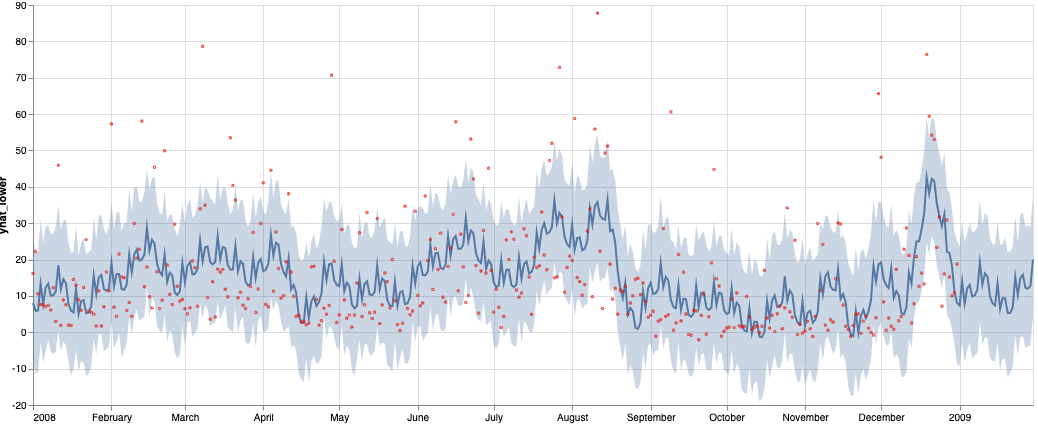
This generates a pandas dataframe with a forward-looking forecast for a month, based on past data for the year 2008 for New York City.

dsyhatyhat_loweryhat_upper
3912009-01-2615.837485-1.12745132.935337
3922009-01-2712.255507-4.31690429.076066
3932009-01-2811.985047-3.89463529.361144
3942009-01-2912.829259-3.57005928.911738
3952009-01-3020.0246414.54343137.593828

Finally, to see show how Ibis can support multiple backends, including pandas as an ibis backend, build an Altair chart for the forecast output dataframe to see what the forecast looks like. Use Altair’s compound chart functionality to overlay the original Ibis expression for the past data, with the error bounds and the forecast trend line.

1connection = ibis.pandas.connect({'forecast': forecast })
2table = connection.table('forecast')
3
4line = alt.Chart(table).mark_line().encode(
5 x='ds:T',
6 y='yhat:Q'
7)
8
9band = alt.Chart(table).mark_errorband().encode(
10 x='ds:T',
11 y='yhat_lower:Q',
12 y2='yhat_upper:Q'
13)
14
15points = alt.Chart(get_delay_ts('New York')).mark_point(size=2, color='red').encode(
16x='ds:T',
17y='y:Q')
18
19(band+line+points).properties(width=1000, height=400)

The generated chart shows the past data and extends out by a month to show predicted arrival delay.

The above forecast is for a single city. If you want to create arrival delay forecasts for multiple cities in parallel, you can use frameworks like Dask or Ray that allow distributed execution.

Parallelizing the Forecasts

In the example above, the function get_delay_ts returns a single time series for a city. You may want to compute arrival delay forecasts for a large number cities. Each prophet forecast takes approximately 1-2 seconds.

Let’s see how many forecasts you need to generate:

1t.dest_city.nunique().execute()
2
3#this should return the following, for the public flights dataset used above
4290

At about 1-2 seconds per Prophet forecast, running these serially could take anywhere from 5-10 minutes**.** Because the time series for arrival delays for each city is independent, parallelization can speed up the process.

Using Dask

Use Dask to parallelize this operation. First, make sure you have Dask installed in your Python environment:

1conda install -c conda-forge dask

Now, modify the method slightly to get the time series of daily arrival delays for a city. Make the city an optional parameter, and group by the city.

1def get_delay_ts(city: str = None):
2 ds=t.dep_timestamp.truncate('D').name('ds')
3 y = t.depdelay.mean().name('y')
4
5 filters = [ds.notnull()]
6
7 if city is not None:
8 filters.append(t.dest_city == city)
9
10 expr = t.filter(filters).group_by([ds, t.dest_city]).aggregate(y)
11 return expr

Try this modified method to see if it works correctly without a parameter for the city name.

1 print(get_delay_ts().compile())
2
3 #This will return the following. Passing in a city parameter will filter by the city
4 SELECT DATE_TRUNC(DAY, "dep_timestamp") AS ds, "dest_city",
5 avg("depdelay") AS y
6 FROM flights_donotmodify
7 WHERE DATE_TRUNC(DAY, "dep_timestamp") IS NOT NULL
8 GROUP BY ds, dest_city

Now, use Dask to parallelize this operation.

1from dask import delayed
2from dask.distributed import Client, progress
3
4def get_forecast_for_ts(city, ts):
5 print(f'Computing forecast for {city}')
6 m = Prophet()
7 m.add_seasonality(name='yearly', period=365, fourier_order=10)
8 m.fit(ts)
9 future = m.make_future_dataframe(periods=7, freq='D')
10 fcst = m.predict(future)
11 return fcst
12
13#This function creates an input dataframe for Prophet, keyed by city
14#and executes the prophet forecast in parallel over a specified number of workers
15def get_forecasts_dask(city:str = None):
16 input_df = get_delay_ts(city=city).execute()
17
18 #Change n_workers as needed for the machine you're running on (number of cores)
19 client = Client(threads_per_worker=1, n_workers=16)
20
21 #Use dask delayed, to create an array of deferred calls to the forecast method, splitting the above result dataframe by city
22 fcsts = [delayed(get_forecast_for_ts)(city=k, ts=v[['ds','y']]) for k, v in input_df.groupby('dest_city')]
23
24 #Run the forecasts in parallel
25 try:
26 forecasts = delayed(fcsts).compute()
27 return forecasts
28 except Exception as e:
29 print(f"Unexpected error {e}")
30 finally:
31 client.close()

You are ready to run parallelized forecasting. You have materialized the data for all cities in a single call, split the resulting dataframe by city, and handed it off to Dask to compute the forecast, returning an array with all the forecasts.

1%%time
2dask_forecasts=get_forecasts_dask()

Once you start the run, you can examine the Dask UI at localhost:8787 (assuming you can access it on the running machine), where you can see the entire process. With 16 cores (as specified in the call to Dask), forecasts for 288 cities complete in approximately 75-90 seconds---a 3-6x increase in speed.

1CPU times: user 27 s, sys: 1.91 s, total: 28.9 s
2Wall time: 1min 31s

Using Ray

Next, let’s use Ray, a distributed execution engine for Python. Ray is similar to Dask, but more specifically targeted at machine learning and deep learning workflows, and can be used to parallelize existing Python code. To get started, install Ray.

1pip install -U ray

Next, modify the methods used previously for use with Ray. In particular, declare the Prophet forecasting method to be a Ray remote method, which allows Ray to execute it on a cluster or a set of cores in parallel.

1import ray
2
3#the below decorator allows Ray's runtime to execute multiple instances of it in parallel
4@ray.remote
5def get_forecast_for_ts(city, ts):
6 print(f'Computing forecast for {city}')
7 m = Prophet()
8 m.add_seasonality(name='yearly', period=365, fourier_order=10)
9 m.fit(ts)
10 future = m.make_future_dataframe(periods=7, freq='D')
11 fcst = m.predict(future)
12 return fcst
13
14#This method is very similar to the Dask method, except for how Ray is invoked
15def get_forecasts_ray(city:str = None):
16 ray.shutdown()
17 ray.init(ignore_reinit_error=True, log_to_driver=False, logging_level='INFO')
18
19 #Use Ibis to get the specific set of fuel locations to run the forecast on
20 input_df = get_delay_ts(city=city).execute()
21
22 #Create an array of deferred forecast objects that Ray will evaluate in parallel
23 fcsts = [get_forecast_for_ts.remote(city=k, ts=v[['ds','y']]) for k, v in input_df.groupby('dest_city')]
24 return ray.get(fcsts)

This starts a Ray distributed computation, similar to Dask. Ray is slightly faster for this same task.

1CPU times: user 16.4 s, sys: 762 ms, total: 17.1 s
2Wall time: 1min 23s
12020-08-30 16:20:02,762 INFO resource_spec.py:231 -- Starting Ray with 29.54 GiB memory available for workers and up to 14.77 GiB for objects. You can adjust these settings with ray.init(memory=<bytes>, object_store_memory=<bytes>).
22020-08-30 16:20:03,142 INFO services.py:1193 -- View the Ray dashboard at localhost:8265
3
4CPU times: user 16.4 s, sys: 762 ms, total: 17.1 s
5Wall time: 1min 23s