DTensor Tensor Parallel Accuracy Issue#
During reinforcement learning (RL) post-training, maintaining accuracy is both critical and challenging. Minor numerical deviations can propagate and amplify across policy updates, ultimately distorting reward signals and affecting convergence. Consequently, understanding and mitigating accuracy issues is central to ensuring consistent and reliable training behavior in large-scale distributed RL settings.
Observed Accuracy Issues Under Tensor Parallelism with DTensor Backend#
During our development, we identified that the tensor parallel (TP) strategy can be a significant factor contributing to accuracy problems.
We have encountered several accuracy issues related to TP in DTensor, including:
For policy models: We observed severe
token_mult_prob_errorspikes when TP was enabled during post-training of a Qwen3 dense model (e.g., Qwen/Qwen3-4B-Instruct-2507 · Hugging Face), indicating a significant difference between the training and inference engines.For reward models: The reward model exhibited large discrepancies under different TP configurations.
For overall model training performance: Using a \(TP > 1\) configuration often leads to degraded downstream performance when utilizing either DTensorPolicyWorker or DTensorPolicyWorkerV2.
Misalignment between Training and Inference for Policy Models#
Using Qwen/Qwen3-4B-Instruct-2507 as an example, Figure 1 illustrates the token_mult_prob_error observed during training. We applied a time-weighted exponential moving average (EMA) smoothing method and used a logarithmic scale on the Y-axis for better visualization.
The token_mult_prob_error metric measures the discrepancy between the inference engine and the training engine when processing the same sample. It is defined as follows:
In general, generation logprobs and policy logprobs should align closely, resulting in a token_mult_prob_error value near 1.0. In our development, when this metric exceeds 1.05, we consider it indicative of a potential framework issue that warrants further investigation.
As shown in Figure 1, numerous spikes can be observed during training. Occasional spikes are acceptable if the token_mult_prob_error quickly returns to around 1.0. However, in this case, even with EMA smoothing applied, the figure reveals an overall upward trend, which is unacceptable and indicates a persistent misalignment between the training and inference behaviors.
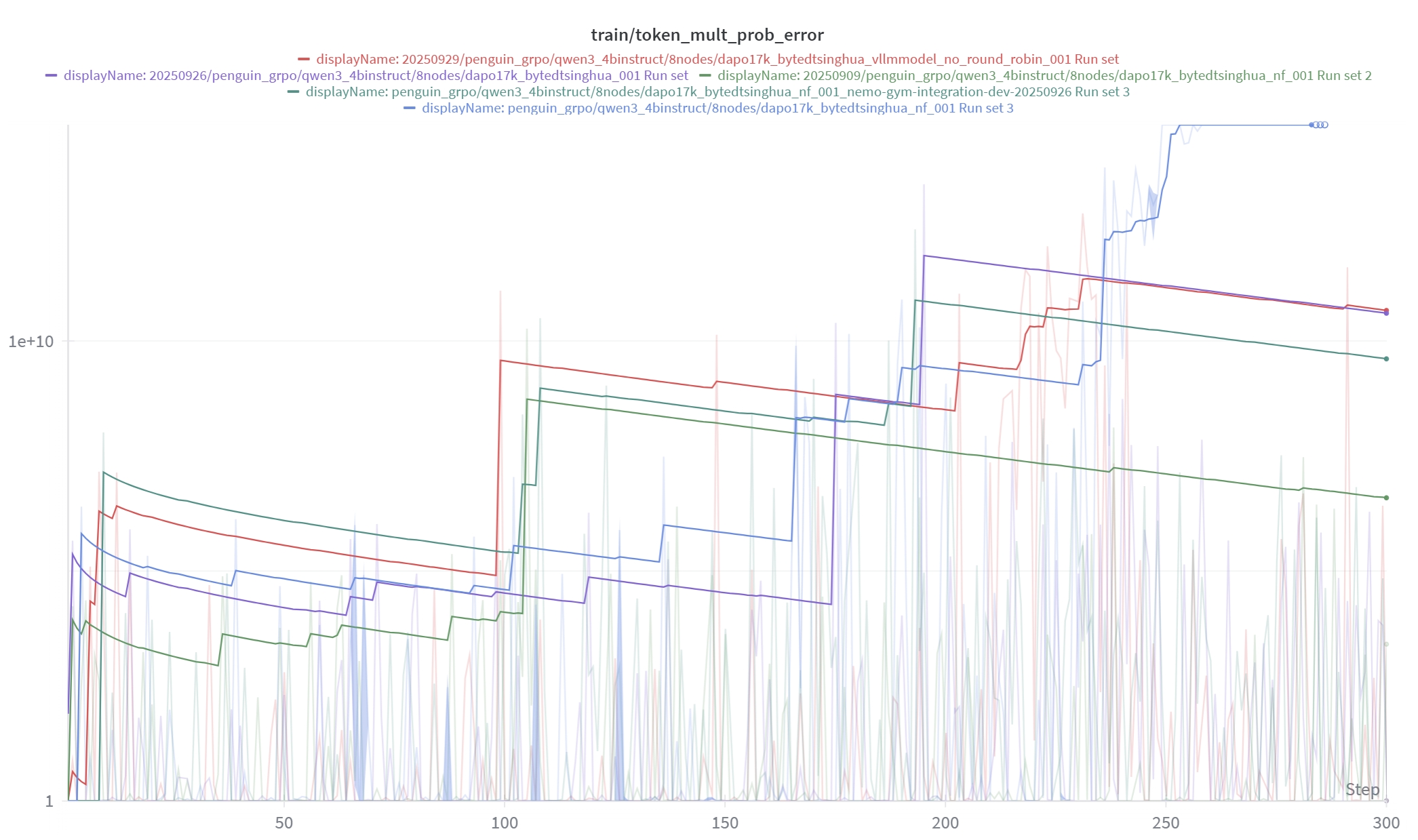
Fig 1: The token_mult_prob_error of Qwen3-4B
Discrepancies Across TP Configurations in Reward Modeling#
For the reward model, different TP plans lead to slight but noticeable inconsistencies in the validation loss. As summarized in Table 1, the loss values vary across TP settings, with TP=4 showing a larger deviation from the TP=1 baseline than TP=2 or TP=8. This suggests that the choice of TP configuration can subtly affect the numerical behavior of the reward model, even when all other training conditions are held constant.
To investigate whether mixed‑precision arithmetic was a major contributor, autocast was disabled in a separate set of experiments so that computations were performed in full precision. However, the validation losses with and without autocast are essentially identical for all TP settings, indicating that mixed‑precision itself is not the root cause of the discrepancy. Instead, these results imply that the primary source of inconsistency lies in how different TP plans partition and aggregate computations across devices, rather than in precision loss from autocast.
TP=1 |
TP=2 |
TP=4 |
TP=8 |
|
|---|---|---|---|---|
With autocast |
0.6035 |
0.6010 |
0.5864 |
0.6021 |
W/O autocast |
0.6035 |
0.6010 |
0.5864 |
0.6021 |
Table 1: The validation loss of reward model training
Overall Performance Degradation Under Tensor Parallelism#
Figure 2 and Figure 3 present the reward curves and validation accuracy curves for multiple runs under different tensor parallel (TP) configurations. We also apply EMA smoothing for better visualization. The mismatch between the policy engine and the generation engine can lead to degraded downstream accuracy. This issue is most evident in the blue and purple curves, whose corresponding experiments are also the most abnormal cases observed in Figure 1.
Combining the three images for observation, it is not necessarily true that abnormal token_mult_prob_error leads to abnormal reward and validation accuracy. This occurs for several reasons:
Spike pattern instead of continuous growth: In many runs,
token_mult_prob_errorshows frequent spikes rather than a monotonically increasing trend, indicating that training is unstable but not fundamentally broken.Stochastic occurrence of spikes: The abnormal
token_mult_prob_erroris itself unstable; even with the same batch of data, spikes may not appear in every run.Dilution effect with large datasets: When the dataset is sufficiently large and no critical samples are repeatedly affected, these extreme but sporadic spikes may have limited impact on aggregate metrics, so the final reward and validation accuracy may not exhibit significant deviations.
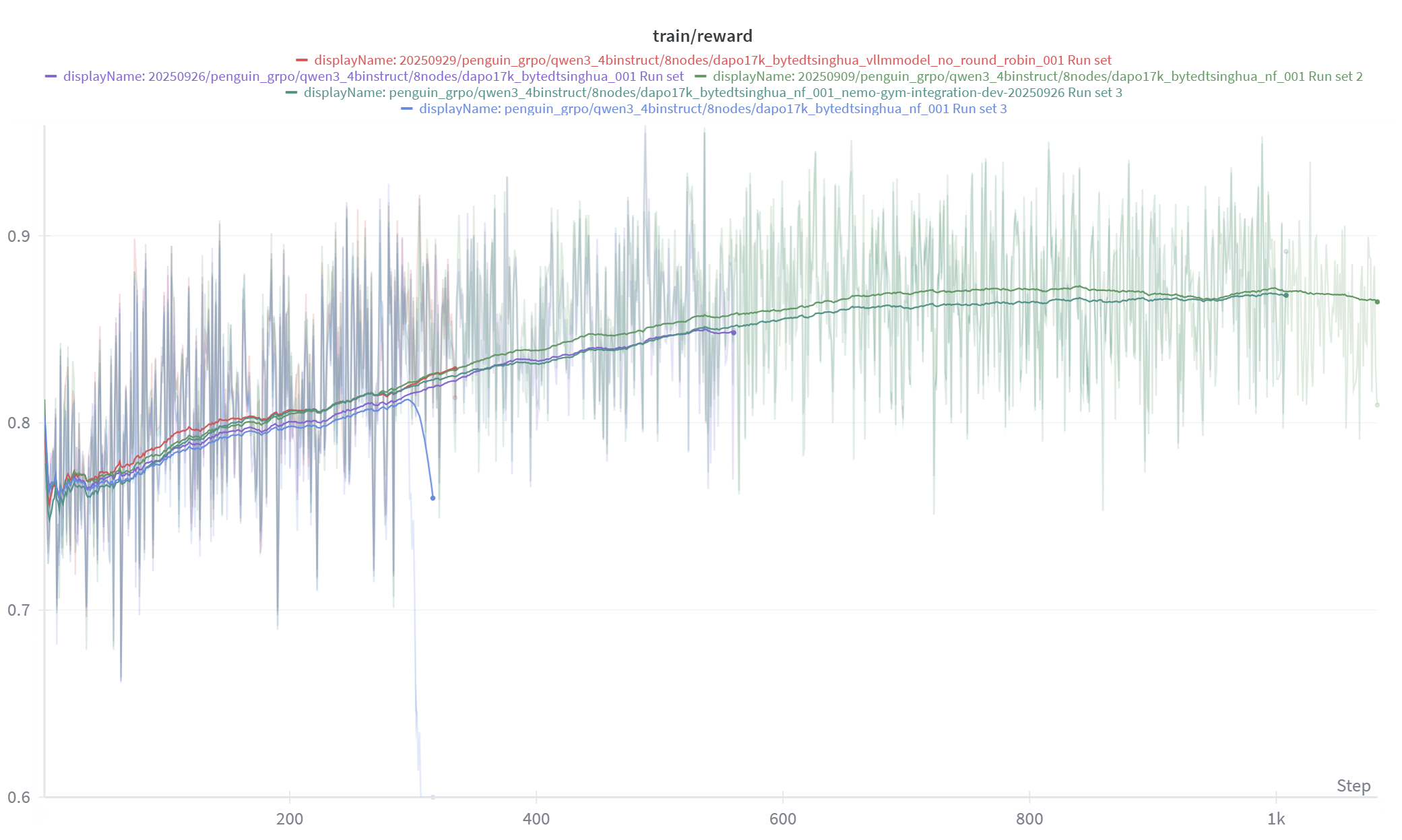
Fig 2: The reward of Qwen3-4B
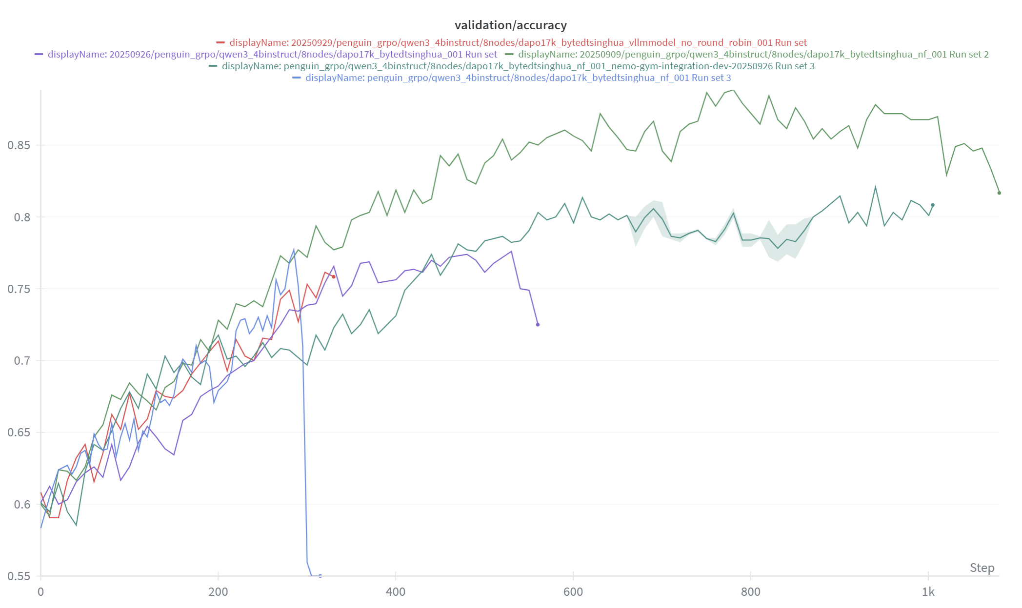
Fig 3: The validation accuracy of Qwen3-4B
However, such training instability is unacceptable for an RL training framework, so we aim to identify and eliminate the underlying issues. There are several challenges in resolving this problem:
Model dependence: The issue is model-dependent rather than universal. For example, this phenomenon is observed on Qwen3-4B but not on Llama-3.1-8B-Instruct.
Poor reproducibility: Abnormal spikes in
token_mult_prob_errorcannot be reproduced reliably. Even with the same batch of data and identical configurations, repeated runs may yield different outcomes.
Our in-depth analysis across multiple models and runs indicates that this behavior does not stem from a single root cause but rather from the interaction of several subtle factors. Taken together, these findings point to a small set of dominant contributors that consistently correlate with the observed instability. Our investigation revealed multiple contributing factors, with the most significant being:
Batch-variant kernels, which can produce inconsistent results across microbatches.
A row-wise TP plan, as row-wise partitioning can introduce additional numerical inconsistencies during distributed computation.
Batch-Variant Kernels#
In RL training, log probabilities are typically computed for samples drawn from the old policy, denoted as prev_logprobs. The same samples are then evaluated under the current policy being optimized, yielding current_logprobs. Using these two quantities, we compute the ratio between the current and previous policies as follows:
This ratio is the standard importance ratio used in off-policy RL to reweight returns when the data are collected under an older behavior policy. In on-policy training, this ratio should be exactly 1. However, in our experiments, we observed cases where the ratio deviates from 1, indicating a mismatch between the intended on-policy setting and the actual behavior of the system. Figure 4 and Figure 5 illustrate this phenomenon by showing the mismatch between prev_logprobs and current_logprobs under TP=4, as well as the reward curves under TP=4 and TP=1 for the deepseek-ai/DeepSeek-R1-Distill-Qwen-7B model.
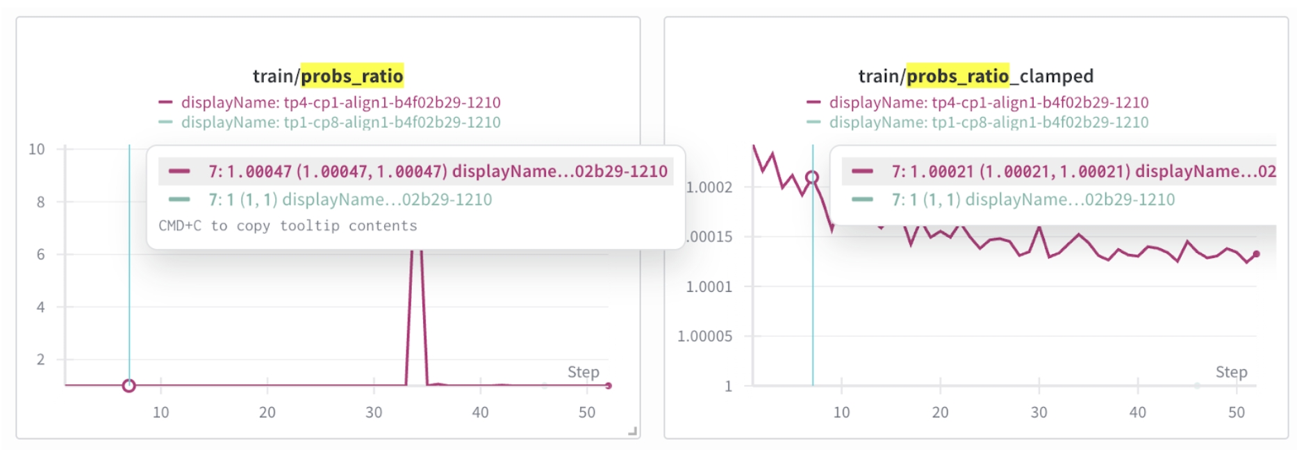
Fig 4: The mismatch of prev_logprobs and current_logprobs under TP=4
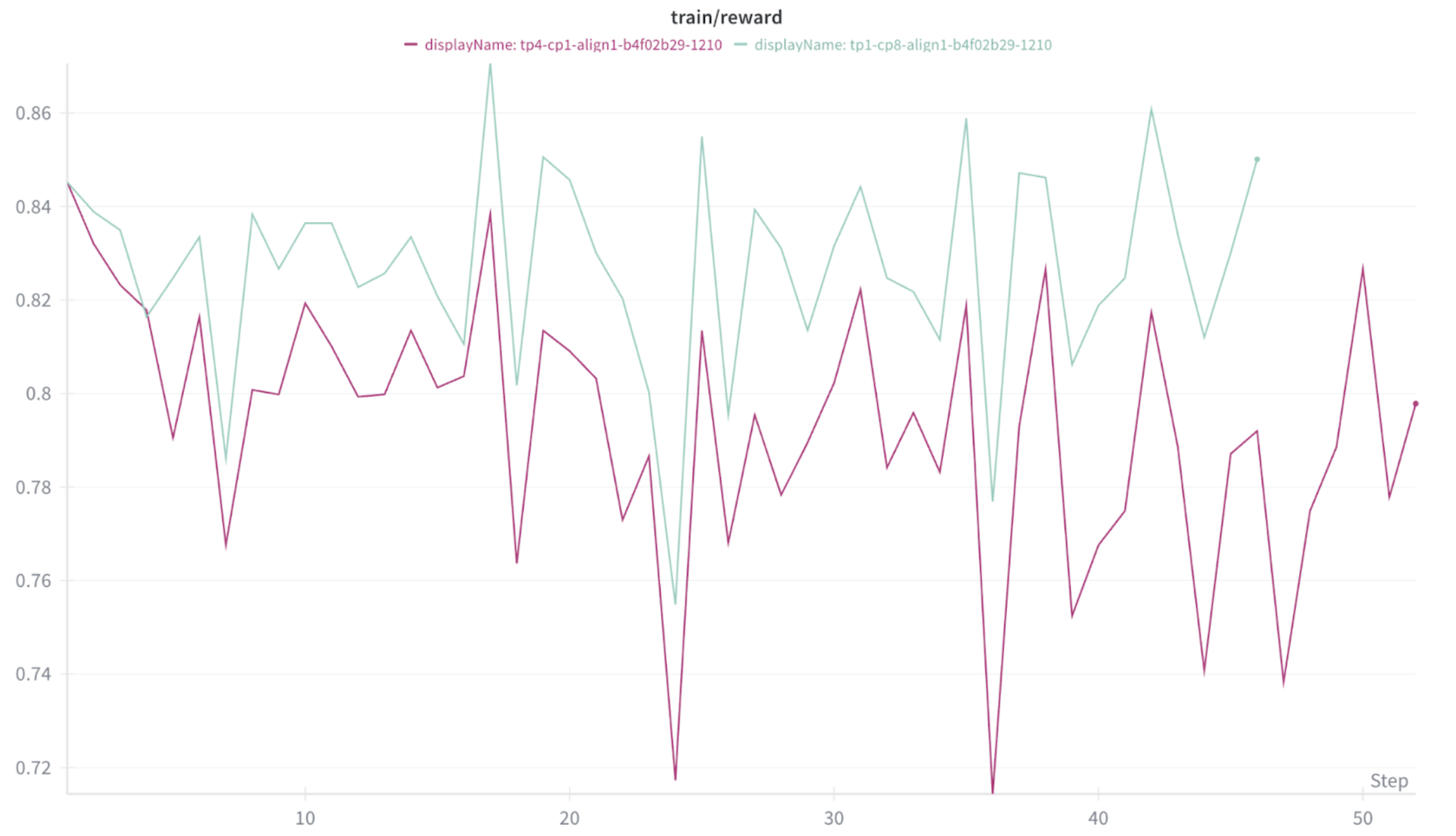
Fig 5: The reward of deepseek-ai/DeepSeek-R1-Distill-Qwen-7B under TP=4 and TP=1
Root Cause#
Upon further investigation, the discrepancy between current_logprobs and prev_logprobs was traced to a mismatch between train_micro_batch_size and logprob_batch_size, which caused the model to behave differently for the same logical samples under different effective batch sizes. This behavior is a typical manifestation of batch-variant kernels, where the numerical outputs of certain operators depend not only on the input tensors themselves but also on how those tensors are grouped into batches or microbatches.
In batch-variant kernels, low-level implementation details—such as parallel reduction order, tiling strategy, fused-kernel heuristics, or algorithm selection conditioned on batch size or sequence layout—can change when the batch size changes, leading to small but systematic numerical differences in the computed logprobs. When train_micro_batch_size and logprob_batch_size are inconsistent, the same token sequence may traverse slightly different computational paths during training and logprob evaluation, resulting in current_logprobs != prev_logprobs and importance-sampling ratios that deviate from 1, even in nominally on-policy settings.
After aligning train_micro_batch_size and logprob_batch_size so that the same samples are processed with identical effective batch configurations, the importance-sampling ratio (probs_ratio) becomes 1 as expected, and the observed accuracy issues disappear. This confirms that the mismatch was caused by batch-dependent numerical variation rather than a conceptual error in the RL objective or data pipeline.
Recommended Solutions#
When using DTensor with TP > 1, or when probs_ratio != 1 is observed in an on-policy setting, the following mitigation strategies are recommended to restore numerical consistency and stabilize training:
Align micro-batch sizes: Configure
train_micro_batch_sizeandlogprob_batch_sizeto be exactly equal so that both the training forward pass and the logprob evaluation traverse identical kernel configurations and batching patterns. This alignment minimizes batch-variant behavior in underlying kernels and ensures thatcurrent_logprobsandprev_logprobsare computed under the same numerical conditions, which in turn drivesprobs_ratioback toward 1.Force an on-policy ratio: In strictly on-policy scenarios, enable the
loss_fn.force_on_policy_ratioflag to explicitly setprobs_ratioto 1 during loss computation. This option is appropriate only when the data are guaranteed to be collected from the current policy and the theoretical importance-sampling ratio should be exactly 1; under these assumptions, clamping the ratio removes spurious numerical noise introduced by minor logprob mismatches while preserving the correctness of the training objective.
Row-Wise TP Plan#
Row-wise and column-wise parallelism are two common ways to split a large linear layer across multiple devices. They differ in which dimension of the weight matrix is partitioned and how the partial results are combined.
Consider a linear layer \(y=xW^T\) with \( W^T \in \mathbb{R}^{d_{\text{in}} \times d_{\text{out}}},\quad x \in \mathbb{R}^{d_{\text{in}}},\quad y \in \mathbb{R}^{d_{\text{out}}}. \).
Row-wise parallel (TP = 2)
In row-wise parallelism, we split \(W^T\) by rows (input dimension) into two blocks:
We also split the input:
Each GPU holds its own input slice and weight slice, and computes: \(y_1 = x_1W_1^T,\quad y_2 =x_2W_2^T\), then we sum the partial outputs: \(y = y_1 + y_2\)
Column-wise parallel (TP = 2)
In column-wise parallelism, we split (W^T) by columns (output dimension) into two blocks:
Each GPU gets the full input \(x\) and computes: \(y_1 = xW_1^T ,\quad y_2 = xW_2^T\), then we concatenate along the output dimension: \(y = \left[ y_1, y_2 \right]\).
Root Cause#
Our analysis shows that the row-wise (colwise) tensor parallel (TP) plan is a primary driver of the observed spikes in metrics and the instability of the reward model when TP is enabled. Row-wise tensor parallelism inevitably introduces cross-device reductions on the output activations. In the row-wise case, each rank produces a partial output \(y_i\), and these partial results must be summed across GPUs to form the final \(y=∑_iy_i\). Although floating‑point addition is mathematically associative, its implementation in finite precision is non-associative, so changing the summation order can lead to different numerical results, and the accumulated error can grow over long reduction chains. This makes large distributed reductions—such as the cross‑GPU adds required by row-wise TP—particularly vulnerable to run‑to‑run variability and small but systematic drift.
By contrast, when the entire reduction is executed within a single device and on the same tensor core pipeline, the execution order and kernel implementation are typically fixed for a given problem size, which tends to yield deterministic and more numerically stable results for repeated runs with the same inputs. In other words, on a single GPU, the hardware and library stack generally ensure that the same matmul and accumulation schedule is reused, so the rounding pattern is at least consistent, even if it is not perfectly exact. However, once the computation is split across multiple GPUs, the final sum depends on the collective communication pattern (for example, ring or tree AllReduce), thread scheduling, and low‑level communication libraries. These factors are not guaranteed to be deterministic and can change the effective addition order, leading to additional rounding error and small cross‑rank discrepancies in the aggregated outputs.
Recommended Solutions:#
To mitigate the numerical instability introduced by row-wise TP (especially the cross‑GPU reductions on attention and MLP outputs), we recommend using a numerically more stable TP plan that avoids cross‑rank summations. Instead of summing partial outputs across GPUs, the stable plan favors column-wise sharding with local outputs, so that each rank produces a complete, independent slice of the logits and no inter‑GPU add is required on these critical paths.
Below is an example of how the default plan can be adjusted into a more numerically stable configuration. More details can refer to NeMo-RL PR! 1235.
custom_parallel_plan = {
    "model.embed_tokens": RowwiseParallel(input_layouts=Replicate()),
    "model.layers.*.self_attn.q_proj": ColwiseParallel(),
    "model.layers.*.self_attn.k_proj": ColwiseParallel(),
    "model.layers.*.self_attn.v_proj": ColwiseParallel(),
    "model.layers.*.self_attn.o_proj": RowwiseParallel(),
    "model.layers.*.mlp.up_proj": ColwiseParallel(),
    "model.layers.*.mlp.gate_proj": ColwiseParallel(),
    "model.layers.*.mlp.down_proj": RowwiseParallel(),
    "lm_head": ColwiseParallel(output_layouts=Shard(-1), use_local_output=False),
}

numerical_stable_parallel_plan = {
    "model.embed_tokens": RowwiseParallel(input_layouts=Replicate()),
    "model.layers.*.self_attn.q_proj": ColwiseParallel(),
    "model.layers.*.self_attn.k_proj": ColwiseParallel(),
    "model.layers.*.self_attn.v_proj": ColwiseParallel(),
    "model.layers.*.self_attn.o_proj": ColwiseParallel(
        input_layouts=Shard(-1),
        output_layouts=Replicate(),
        use_local_output=True,
    ),
    "model.layers.*.mlp.up_proj": ColwiseParallel(),
    "model.layers.*.mlp.gate_proj": ColwiseParallel(),
    "model.layers.*.mlp.down_proj": ColwiseParallel(
        input_layouts=Shard(-1),
        output_layouts=Replicate(),
        use_local_output=True,
    ),
    "lm_head": ColwiseParallel(output_layouts=Shard(-1), use_local_output=False),
}
Additional Observations and Insights#
Beyond the TP-related issues discussed above, our experiments also highlight that accuracy in RL training is influenced by a broad set of numerical factors, including attention backends (such as SDPA and flash attention2), GPU architectures (such as Ampere vs Hopper), and arithmetic precision settings (such as BF16/FP16/FP8/FP32). Different inference and training engines often implement kernels using distinct implementation methods, which naturally introduce small discrepancies in floating‑point results even when the high‑level math is identical. As a result, two systems that are “functionally equivalent” may still produce slightly different logprobs, rewards, or validation metrics.
Figure 6 reports the KL divergence between the logits produced by the Hugging Face stack and those produced by NeMo‑RL for the same input sequence. The plot shows that, even with identical data and model weights, the resulting logit distributions differ noticeably across the two execution engines. In our experiments, similar behavior appeared when varying attention implementations and hardware configurations, where we consistently observed measurable numerical discrepancies, although we did not attempt to systematically eliminate every such source of variation.
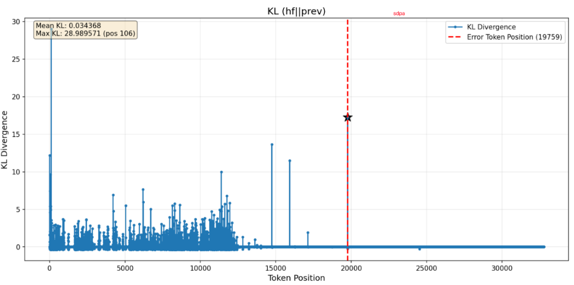
Fig 6: The KL divergence between hugging face and nemorl
The broader research community has proposed multiple strategies to mitigate these issues. We have referred to a list of publications:
In our current work, we treat these effects primarily as background noise and focus on TP‑induced misalignment that has a clear and actionable impact on RL training. A more exhaustive treatment—such as systematically unifying attention backends, enforcing TP‑invariant kernels, or integrating compensated summation into critical paths—is left as future engineering work informed by the aforementioned research directions.