Profiling Tools#
This tutorial introduces tools and techniques that can be used to measure the performance of PVA applications. Profiling tools can be used to determine if the developed application meets the performance goals and to get hints about potential performance bottlenecks.
Three profiling techniques are introduced in this tutorial. Each tool has specific advantages to meet the needs of the PVA developer.
NVIDIA Nsight™ Systems: A visual performance analysis tool that does not need any code instrumentation.
Timestamp Counter (TSC): A performance counter that can be used to instrument the device code to measure how many VPU cycles are spent to execute certain code blocks.
Profiling Stream: A profiling extension of the standard
cupva::Streamthat collects the CmdProgram and VPU Executable performance statistics in nanoseconds resolution. The profiling stream is currently only available for the C++ API.
We profile the three versions of the unsharp masking algorithm we have developed in the previous tutorials. The non-vectorized reference code developed in RDF Halo Configuration Tutorial, the vectorized code developed in VPU Programming Basics Tutorial and the optimized version developed in Optimizing VPU Programs Tutorial is used. Three Executables and CmdPrograms are created using the aforementioned device code versions. The CmdPrograms are submitted as a batch in the host code as follows:
Three executables are declared first:
constexpr int32_t PROGRAM_COUNT{3};
PVA_DECLARE_EXECUTABLE(profiling_nonvectorized_dev)
PVA_DECLARE_EXECUTABLE(profiling_vectorized_dev)
PVA_DECLARE_EXECUTABLE(profiling_optimized_dev)
Executables and CmdPrograms are created and submitted:
        std::vector<Executable> execs;
        execs.emplace_back(Executable::Create(PVA_EXECUTABLE_DATA(profiling_nonvectorized_dev),
                                              PVA_EXECUTABLE_SIZE(profiling_nonvectorized_dev)));
        execs.emplace_back(Executable::Create(PVA_EXECUTABLE_DATA(profiling_vectorized_dev),
                                              PVA_EXECUTABLE_SIZE(profiling_vectorized_dev)));
        execs.emplace_back(Executable::Create(PVA_EXECUTABLE_DATA(profiling_optimized_dev),
                                              PVA_EXECUTABLE_SIZE(profiling_optimized_dev)));
        std::vector<CmdProgram> progs;
        for (int i = 0; i < PROGRAM_COUNT; i++)
        {
            progs.emplace_back(CmdProgram::Create(execs[i]));
        }
        CmdStatus status[PROGRAM_COUNT + 1];
        stream.submit({&progs[0], &progs[1], &progs[2], &rf}, status);
The remaining steps for configuring the parameters and data flows and creating streams and fences are skipped since they are very similar to the previous tutorials.
Three executables are declared first:
#define PROGRAM_COUNT 3
PVA_DECLARE_EXECUTABLE(profiling_nonvectorized_dev)
PVA_DECLARE_EXECUTABLE(profiling_vectorized_dev)
PVA_DECLARE_EXECUTABLE(profiling_optimized_dev)
    int createdExecutableCount = 0;
    cupvaExecutable_t execs[PROGRAM_COUNT];
    CHECK_ERROR_GOTO(CupvaExecutableCreate(&execs[0], PVA_EXECUTABLE_DATA(profiling_nonvectorized_dev),
                                           PVA_EXECUTABLE_SIZE(profiling_nonvectorized_dev)),
                     err, ExecutableCreateFailed);
    createdExecutableCount++;

    CHECK_ERROR_GOTO(CupvaExecutableCreate(&execs[1], PVA_EXECUTABLE_DATA(profiling_vectorized_dev),
                                           PVA_EXECUTABLE_SIZE(profiling_vectorized_dev)),
                     err, ExecutableCreateFailed);
    createdExecutableCount++;

    CHECK_ERROR_GOTO(CupvaExecutableCreate(&execs[2], PVA_EXECUTABLE_DATA(profiling_optimized_dev),
                                           PVA_EXECUTABLE_SIZE(profiling_optimized_dev)),
                     err, ExecutableCreateFailed);
    createdExecutableCount++;

    int createdCmdProgramCount = 0;
    cupvaCmd_t progs[PROGRAM_COUNT];
    for (int i = 0; i < PROGRAM_COUNT; i++)
    {
        CHECK_ERROR_GOTO(CupvaCmdProgramCreate(&progs[i], execs[i]), err, CmdProgramCreateFailed);
        createdCmdProgramCount++;
    }
Executables and CmdPrograms are created and submitted:
    int createdExecutableCount = 0;
    cupvaExecutable_t execs[PROGRAM_COUNT];
    CHECK_ERROR_GOTO(CupvaExecutableCreate(&execs[0], PVA_EXECUTABLE_DATA(profiling_nonvectorized_dev),
                                           PVA_EXECUTABLE_SIZE(profiling_nonvectorized_dev)),
                     err, ExecutableCreateFailed);
    createdExecutableCount++;

    CHECK_ERROR_GOTO(CupvaExecutableCreate(&execs[1], PVA_EXECUTABLE_DATA(profiling_vectorized_dev),
                                           PVA_EXECUTABLE_SIZE(profiling_vectorized_dev)),
                     err, ExecutableCreateFailed);
    createdExecutableCount++;

    CHECK_ERROR_GOTO(CupvaExecutableCreate(&execs[2], PVA_EXECUTABLE_DATA(profiling_optimized_dev),
                                           PVA_EXECUTABLE_SIZE(profiling_optimized_dev)),
                     err, ExecutableCreateFailed);
    createdExecutableCount++;

    int createdCmdProgramCount = 0;
    cupvaCmd_t progs[PROGRAM_COUNT];
    for (int i = 0; i < PROGRAM_COUNT; i++)
    {
        CHECK_ERROR_GOTO(CupvaCmdProgramCreate(&progs[i], execs[i]), err, CmdProgramCreateFailed);
        createdCmdProgramCount++;
    }
    cupvaCmd_t const *cmds[PROGRAM_COUNT + 1]  = {&progs[0], &progs[1], &progs[2], &rf};
    cupvaCmdStatus_t status[PROGRAM_COUNT + 1] = {NULL, NULL, NULL, NULL};
    CHECK_ERROR_GOTO(CupvaStreamSubmit(stream, cmds, status, PROGRAM_COUNT + 1, CUPVA_IN_ORDER, -1, -1), err,
                     DeAllocateAllResources);
The remaining steps for configuring the parameters and data flows and creating streams and fences are skipped since they are very similar to the previous tutorials.
NVIDIA Nsight™ Systems#
NVIDIA Nsight Systems is a system-wide performance analysis tool designed to visualize an application’s algorithms, help you identify the largest opportunities to optimize, and tune to scale efficiently across any quantity or size of CPUs and GPUs, from large servers to the smallest system on a chip (SoC).
Nsight Systems can also be used to collect run-time stastics of PVA tasks. It is a great way of visualizing and analyzing the whole processing pipeline, which may potentially involve CPU, GPU or other accelerators on the target device.
Another advantage of Nsight Systems is not needing to instrument the code by adding extra lines. Production-ready applications can be profiled with this non-intrusive tool.
Please refer to Using Nsight Systems with PVA for steps to setup Nsight.
Output#
The application has been launched on the target device with the nsys tool to collect traces as described in NVIDIA Nsight™ Systems.
A report file with the .nsys-rep extension is created when the execution gets completed.
The report can be opened with the nsys-ui GUI tool to display the timeline view.
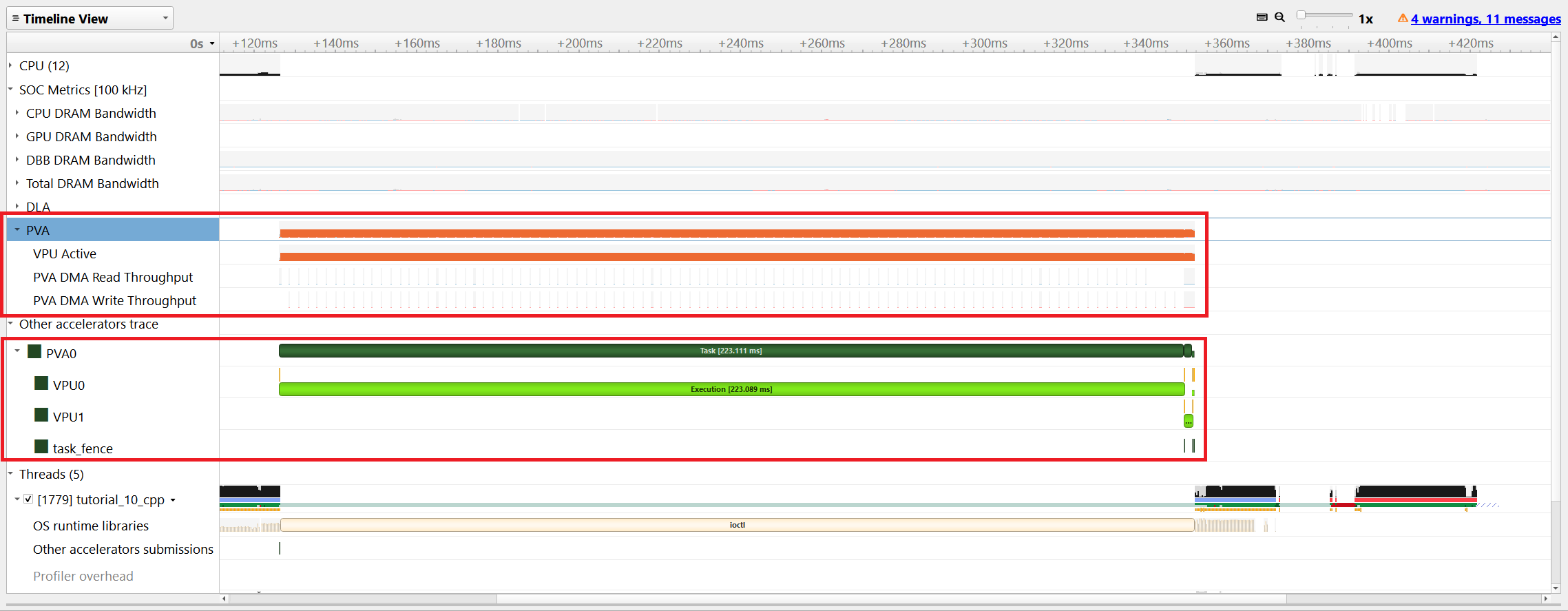
The scheduling of PVA tasks along with other processors and accelerators can be viewed in the Nsight Systems Timeline view. There are two row blocks that display PVA specific profiling information.
The PVA row under the “Other accelerators trace” displays the start and end timing of each PVA task and fence expiration times.
The PVA row under the “SOC Metrics” shows the VPU utilization percentage along with the DMA throughput with 100 kHz sampling frequency.
Note
Displaying SOC Metrics may require a limited distribution release of Nsight Systems.
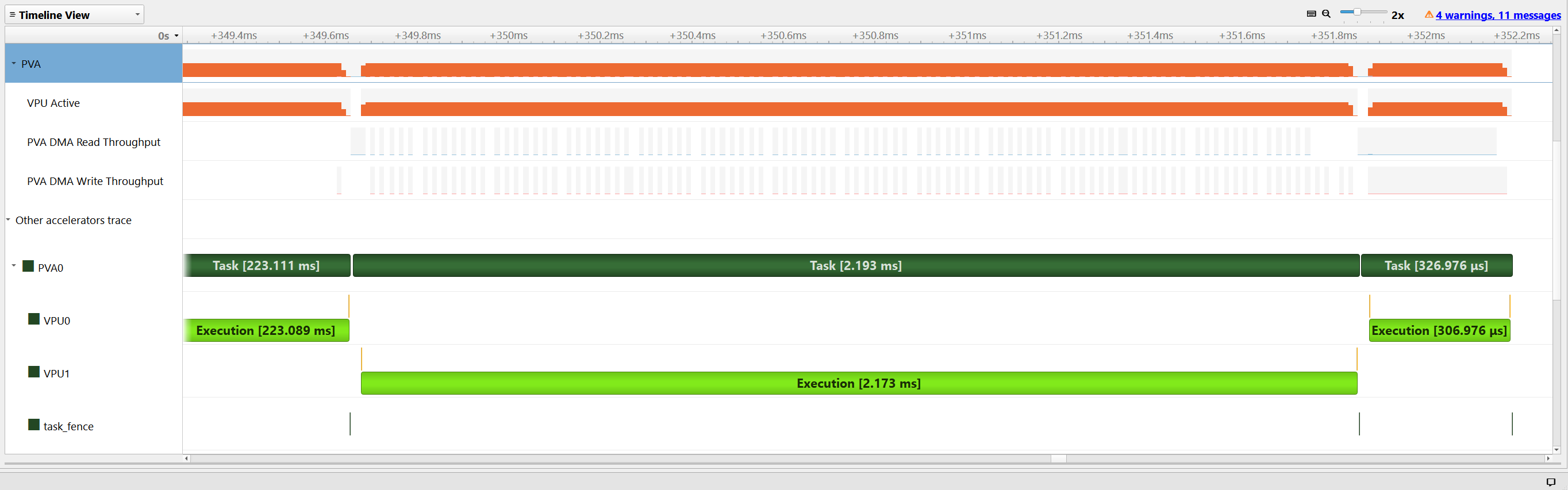
When we zoom closer to the PVA tasks, the back-to-back execution of the three CmdPrograms and the execution duration can be viewed. Rewriting the device code using vector instructions and AGENs provided close to 100x performance boost compared to the reference implementation. The third CmdProgram is ~7x faster than the second one thanks to software pipelining and loop unrolling optimizations.
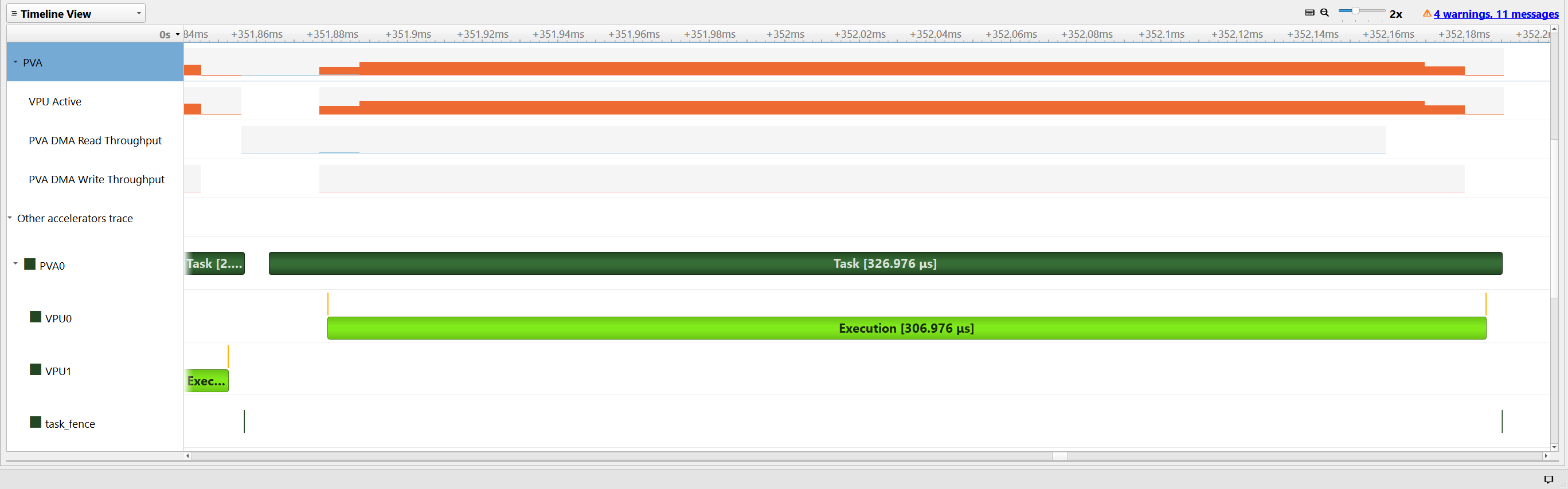
Scheduling of DMA transfers can be seen when we zoom further into the third PVA task. The VPU process starts after the first tiles are transferred to the VMEM as a part of the implemented circular buffering scheme. The task gets completed after the last output tile is written to the DRAM.
Timestamp Counter (TSC)#
TSC is a free-running timestamp counter for performance instrumentation. Each VPU has a 64-bit register that is incremented in each clock cycle once enabled.
The VPU cycles spent between two device-side code lines can be measured. Developers may instrument the code to measure specific algorithm stages or kernel execution times with cycle accuracy. Hence, TSC is useful tool that can used for fine-grained code optimization.
Measured execution times can be displayed conveniently with the VPU printf tool.
TSC register values can be stored in VMEM if you need to measure multiple code blocks or compute statistics from multiple measurements.
#define MAX_TSC_COUNT 100
VMEM(C, uint32_t, TSCBuf, MAX_TSC_COUNT);
TSC should be enabled before starting to take measurements.
    enable_TSC();
    chess_separator_scheduler();
Let’s first measure how many cycles are needed to transfer one tile of input pixels from DRAM to VMEM. We know that when we call
cupvaRasterDataFlowOpen, one tile is transferred to VMEM and a second transfer is started to begin the pipeline. Let’s measure the time for this first transfer.TSCBuf[0] = read_TSCL(); chess_separator_scheduler(); cupvaRasterDataFlowOpen(sourceDataFlowHandler, &inputTileBufferVMEM[0]); chess_separator_scheduler(); TSCBuf[0] = read_TSCL() - TSCBuf[0]; printf("\nSingle Tile Tranfer: %u cycles\n", TSCBuf[0]);
TSC values are read for each tile just before entering the pixel processing loop and after iteration finishes. Counting the filter kernel cycles provides very accurate measurement of the implementation optimality.
        TSCBuf[i] = read_TSCL();
        chess_separator_scheduler();
        for (int32_t y = 0; y < TILE_HEIGHT; y++)
        {
            for (int32_t x = 0; x < TILE_WIDTH; x++)
            {
                int32_t outputPixelAccumulator = 0;
                for (int32_t i = 0; i < KERNEL_HEIGHT; i++)
                {
                    for (int32_t j = 0; j < KERNEL_WIDTH; j++)
                    {
                        int16_t sourcePixel =
                            inputTileBufferVMEM[(srcOffset + (y + i) * srcLinePitch + (x + j)) % srcCircularBufLen];
                        int16_t coefficient = kernel[i * KERNEL_WIDTH + j];

                        outputPixelAccumulator += (int32_t)sourcePixel * coefficient;
                    }
                }
                outputPixelAccumulator           = ((outputPixelAccumulator >> (quantizationBits - 1)) + 1) >> 1;
                outputPixelAccumulator           = max(0, min(outputPixelAccumulator, 255));
                outputTile[y * dstLinePitch + x] = outputPixelAccumulator;
            }
        }
        chess_separator_scheduler();
        TSCBuf[i] = read_TSCL() - TSCBuf[i];
Cycles taken to process a single tile are printed using the VPU printf in all of the three executables.
printf("Non-Vectorized Single Tile Process: %u cycles\n", TSCBuf[0]);
Output#
The cycle counts for tile transfer and processing in a Orin (GEN2) device look like below. Developers can compute the cycles spent to process a single pixel using these measurements and see how close the actual performance is to the speed-of-light (SOL) calculations. For instance, the optimized code took 3250 cycles to process a tile, 64x64 pixels. It corresponds to 0.79 cycles per pixel which is very close to the 0.78 cycles/pixel SOL.
Single Tile Tranfer: 73 cycles
Non-Vectorized Single Tile Process: 2605638 cycles
Vectorized Single Tile Process: 25639 cycles
Optimized Single Tile Process: 3250 cycles
There is an error in the above measurements. It is not possible for a single tile transfer from DRAM to achieve 73 cycles — the memory latency to DRAM is around 10 times this. The cause of the error is that TSC does not increment while the VPU has entered a low power mode waiting for a signal from its DMA engine (WFE_GPI).
To use TSC to measure these time periods, A compile-time setting is provided which changes DMA trigger/sync functions to use polling, rather than entering a low power WFE_GPI state. It is not recommended to use this mode for production code.
It can be set using the PVA SDK’s CMake system (-DPVA_PROFILING_MODE=ON) or directly defined in code
before including cupva_device.h:
#define CUPVA_PROFILING_FLAG 1
#include <cupva_device.h>
It is left as an excercise to the reader to measure true single tile transfer time with this flag set.
Profiling Stream#
Profiling streams enable collection of run-time statistics for the submitted CmdPrograms. It is a very convenient way of measuring the program execution times and overheads without needing any other tool. A minimal change is needed in the host code and the device code remains the same. Currently, this feature is supported only for the cuPVA C++ Host API.
In the host code, a profiling context is created using the
cupva_utils::ProfilingContext::Create()call. Profiling stream uses the profiling context to store the measurements and statistics.cupva_utils::ProfilingContext ctx = cupva_utils::ProfilingContext::Create(); Stream stream = cupva_utils::CreateProfilingStream(ctx);
The three CmdPrograms including the non-vectorized, vectorized, and optimized unsharp masking implementations are submitted to the stream as a batch.
        CmdStatus status[PROGRAM_COUNT + 1];
        stream.submit({&progs[0], &progs[1], &progs[2], &rf}, status);
Collected statistics can be printed when the fence expires. The profiling stream collects statistics for the batch submitted to the stream as well as statistics for the individual CmdPrograms. The
cupva_utils::ProfilingContext::getStatistics()API retrieves the batch and program statistics in nanosecond resolution.cupva_utils::ProfilingStatisticscan be printed using the<<operator. Statistics include minimum, maximum, average, and total time measurements.For the batch statistics, the VPU execution time and the overhead associated with setup stages can be printed.
            cupva_utils::ProfilingStatistics const vpuExecStats =
                ctx.getStatistics(cupva_utils::ProfilingBatchStatType::EXECUTION_TIME);
            cupva_utils::ProfilingStatistics const r5Stats =
                ctx.getStatistics(cupva_utils::ProfilingBatchStatType::TASK_OVERHEAD);
            cupva_utils::ProfilingStatistics const totalBatchStats =
                ctx.getStatistics(cupva_utils::ProfilingBatchStatType::TOTAL_TIME);

            std::cout << std::endl;
            std::cout << std::setw(25) << "Batch profiling statistics:" << std::fixed << std::setprecision(3)
                      << std::endl;
            std::cout << std::setw(25) << "VPU execution:" << std::endl;
            std::cout << vpuExecStats;
            std::cout << std::setw(25) << "Task overhead:" << std::endl;
            std::cout << r5Stats;
            std::cout << std::setw(25) << "Total batch time:" << std::endl;
            std::cout << totalBatchStats;
            std::cout << std::endl;
cupva_utils::ProfilingContext::getStatistics()calls for the CmdPrograms return the individual program statistics. Program setup, execution and tear-down statistics are printed for each program.cupva_utils::ProfilingStatistics progExecStats = ctx.getStatistics(progs[0], cupva_utils::ProfilingProgramStatType::EXECUTION_TIME); cupva_utils::ProfilingStatistics progSetupStats = ctx.getStatistics(progs[0], cupva_utils::ProfilingProgramStatType::SETUP_TIME); cupva_utils::ProfilingStatistics progTeardownStats = ctx.getStatistics(progs[0], cupva_utils::ProfilingProgramStatType::TEARDOWN_TIME); std::cout << std::setw(25) << "Non-vectorized Program profiling statistics:" << std::fixed << std::setprecision(3) << std::endl; std::cout << std::setw(25) << "Program execution:" << std::endl; std::cout << progExecStats; std::cout << std::setw(25) << "Program setup:" << std::endl; std::cout << progSetupStats; std::cout << std::setw(25) << "Program teardown:" << std::endl; std::cout << progTeardownStats; std::cout << std::endl;
Output#
The tutorial application is executed on a Orin (GEN2) device with VPUs running at 1.152 GHz and CPU running at 2.2GHz. The run-time statistics for the batch as well as the individual CmdPrograms are printed. The execution times of the programs on the VPU and the overhead associated with program setup and teardown are measured. Printed program execution times clearly demonstrate the acceleration in the filtering kernel with the vectorization, loop unrolling (factor of 8) and software pipelining optimizations.
Batch profiling statistics:
          VPU execution:
              min time: 313.696 us
              max time: 223725.344 us
          average time: 75408.224 us
            total time: 226224.672 us
          Task overhead:
              min time: 28.256 us
              max time: 34.944 us
          average time: 32.149 us
            total time: 96.448 us
        Total batch time:
              min time: 226338.304 us
              max time: 226338.304 us
          average time: 226338.304 us
            total time: 226338.304 us

Non-vectorized Program profiling statistics:
      Program execution:
              min time: 223725.344 us
              max time: 223725.344 us
          average time: 223725.344 us
            total time: 223725.344 us
          Program setup:
              min time: 23.840 us
              max time: 23.840 us
          average time: 23.840 us
            total time: 23.840 us
        Program teardown:
              min time: 4.416 us
              max time: 4.416 us
          average time: 4.416 us
            total time: 4.416 us

Vectorized Program profiling statistics:
      Program execution:
              min time: 2185.632 us
              max time: 2185.632 us
          average time: 2185.632 us
            total time: 2185.632 us
          Program setup:
              min time: 28.960 us
              max time: 28.960 us
          average time: 28.960 us
            total time: 28.960 us
        Program teardown:
              min time: 4.288 us
              max time: 4.288 us
          average time: 4.288 us
            total time: 4.288 us

Optimized Program profiling statistics:
      Program execution:
              min time: 313.696 us
              max time: 313.696 us
          average time: 313.696 us
            total time: 313.696 us
          Program setup:
              min time: 30.624 us
              max time: 30.624 us
          average time: 30.624 us
            total time: 30.624 us
        Program teardown:
              min time: 4.320 us
              max time: 4.320 us
          average time: 4.320 us
            total time: 4.320 us