

BundleAdjustment#
Overview#
Bundle adjustment jointly refines camera poses and 3D points (tracks) so that the points, projected into the cameras, best match their 2D image observations [1]. It is the refinement step of visual odometry and mapping pipelines.
The operator takes initial poses and points, the 2D measurements, and a per-track visibility bitmask. It returns the refined poses and points, the final cost and the number of iterations used. The entire Levenberg-Marquardt (LM) solve runs on PVA in one submit, with no CPU work between iterations.
Scene model. In this operator, a camera is a pose: camera \(c\) is a rig pose \(P_c\) (world to rig), and
one transform rig2cam (rig to camera) applies to every pose. The bitmask lists the cameras that observe the track
and marks the track as active (refined) or fixed. As in sliding-window bundle adjustment, only a window of up to
five consecutive cameras, set at creation, has its poses refined. The cameras outside the window keep their poses: they
still constrain the points, and they anchor the global frame.
Figure 1 shows the effect on a synthetic scene: the noisy initial points converge onto the ground truth, and the PVA output matches the CPU reference.
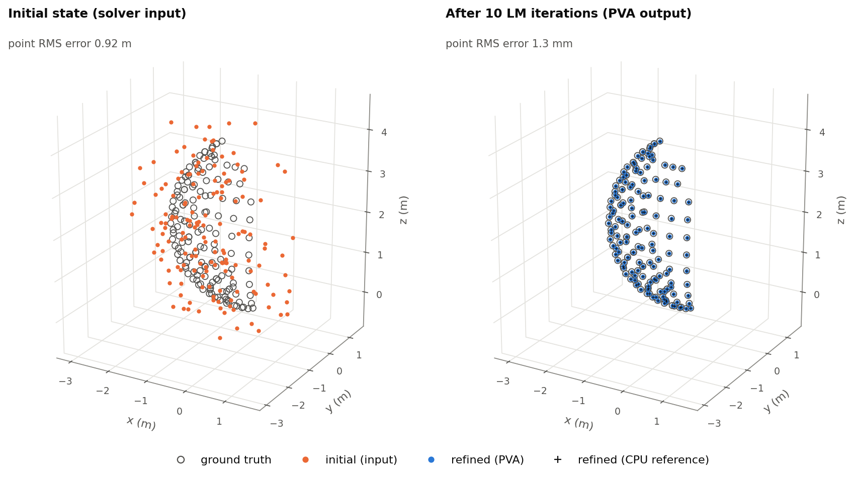
Figure 1: Points before (left) and after (right) bundle adjustment, with RMS errors against ground truth. The scene has 8 cameras on an 8 m ring (cameras 3 to 7 active) and 156 tracks on a sphere. The initial points and active camera positions carry 0.5 m of noise per axis, and the active camera rotations 1°.#
Algorithm Description#
The operator minimizes the robust reprojection cost
where \(\pi\) is the perspective division \((x/z,\ y/z)\), \(m_{pc}\) is the measurement in normalized
image coordinates, and \(\rho(e) = s^2 \ln(1 + e/s^2)\) is the Cauchy loss of the squared error \(e\), with
scale \(s\) = robustifierScaleMeas. An observation whose point has a depth below minDistance (including a
point behind the camera) adds a fixed penalty to the cost but no term to the update.
Each LM iteration linearizes the residuals and solves the normal equations for the pose update \(\delta\mathbf{c}\) (6 DoF per active camera) and the point update \(\delta\mathbf{p}\) (3 per track), with each observation weighted by \(w = \texttt{rinvMeas} / (1 + e/s^2)\):
rinvMeas multiplies every weight, and so both sides of these equations, by the same factor. It does not enter the
reported cost and, in exact arithmetic, does not change the step either.
Each observation links one camera and one point, so \(H_{pp}\) is block-diagonal with one 3×3 block per track. Eliminating the points (Schur complement) leaves the reduced camera system \(S\,\delta\mathbf{c} = g\), at most 30×30, which is solved by Cholesky decomposition. Each track then back-substitutes independently. Fixed tracks are eliminated like the others, but their point update is discarded.
The poses are updated through the SE(3) exponential map. LM damps the system by scaling the diagonal of \(H\) by
\(1 + \lambda\). A step is accepted if \(E\) decreases, which halves \(\lambda\); otherwise \(\lambda\)
grows by 100× [2] (Figure 2). Only
\(\lambda_{\text{init}}\) and maxIterations are submit-time parameters of this schedule.
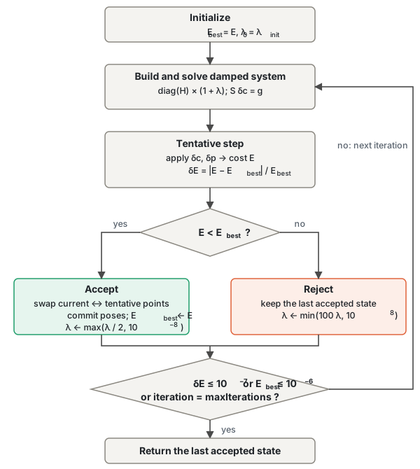
Figure 2: Levenberg-Marquardt routine. A rejected step keeps the last accepted state and retries with a larger \(\lambda\).#
Implementation Details#
Bundle adjustment is not an obvious fit for a SIMD processor. All unknowns are coupled, each track is seen by a different set of cameras, the LM loop makes data-dependent decisions, and up to 20,480 tracks are far more than VMEM holds. Figure 3 shows how the implementation answers each of these:
Independent tracks. After the Schur elimination, the tracks interact only through the reduced camera system \(S\). Each track gets one vector lane, and the tracks stream through VMEM in 128-track tiles, twice per iteration.
Dense instead of sparse. Every tile is processed against every camera, and the visibility bitmask masks the observations that do not exist. The loops are regular and need no gathers; the price is work on unobserved pairs, which the limit of 21 cameras bounds.
Control on the device. The full LM loop, including the accept/reject decision, runs on the VPU, and \(S\) is solved in scalar code between the two passes (Step Rejection Without Rollback).
VMEM independent of the track count. Only the current tiles and the camera-level data stay in VMEM; per-track intermediates go to DRAM between the passes (Dataflow Configuration).
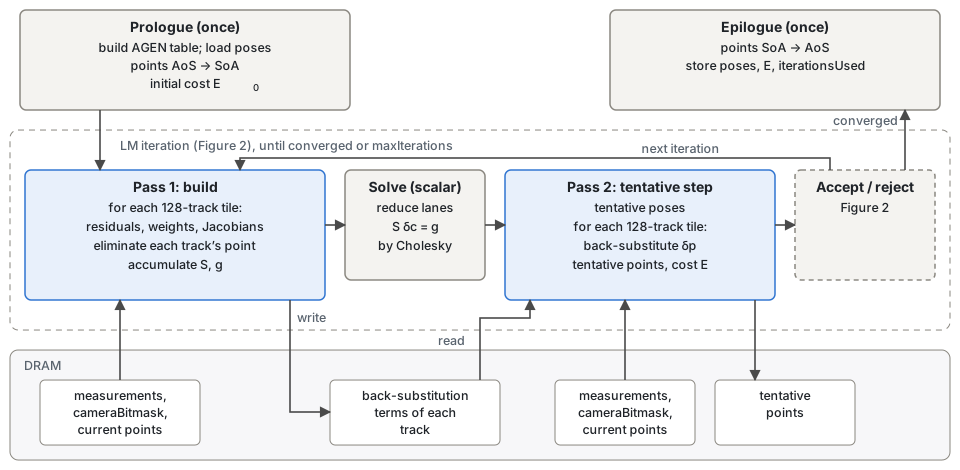
Figure 3: Stages of one submit. Blue boxes stream all tracks in 128-track tiles; arrows to the DRAM band are per-tile DMA transfers. Both passes read the same inputs.#
Data Layout#
The kernels need structure-of-arrays (SoA) data, but the tensors are array-of-structures (AoS). The VPU transposing
load and store (dvfloat_load_transp, vstore_transp) convert between the two when the row pitch is
\(16k + 1\) words, so the DMA writes each AoS tile into a VMEM staging buffer padded to such a pitch (for example,
4-float points to 17 floats). Points are converted once on import and once on export and stay SoA in DRAM during the
loop. Measurements are never converted: the kernels read them from the staging tile with transposing loads.
Dataflow Configuration#
All transfers use SequenceDataFlow. The host fixes each transfer’s size and direction once; on every trigger the VPU
sets the DRAM address (the tile) and the VMEM address (the ping or pong half) with cupvaSQDFUpdateAddr. One handler
per stream and direction therefore serves every tile of every iteration, and the host configures the DMA only once. The
loads of the next tile are issued as soon as those of the current tile complete, so DMA overlaps compute.
Pass 1 stores the back-substitution terms of each track (\(H_{pp}^{-1} b_p\) and \(H_{pp}^{-1} H_{pc}\)) in DRAM scratch, and pass 2 reads them back instead of rebuilding the track.
Step Rejection Without Rollback#
The point state lives in two DRAM buffers, current and tentative. Pass 2 reads the current buffer and writes the tentative one. Acceptance swaps the two base addresses, and rejection discards the tentative buffer, so neither costs any DMA. The poses have a tentative copy in VMEM, which acceptance copies over the current poses.
Buffer Allocation#
The buffers are placed in all four GEN3 VMEM superbanks. GEN2 has no fourth superbank, so the operator does not run on GEN2. Two techniques shape the layout:
Phase reuse. The largest buffer (90 KiB) holds the \(H_{pc}\) blocks of a tile in pass 1, the Cholesky factor in the solve, and the incoming \(H_{pp}^{-1} H_{pc}\) terms in pass 2.
Cross-bank ping-pong accumulation. The reduced camera system is accumulated out of place, alternating between two copies in different superbanks on each update, so a software-pipelined loop never reads and writes the same buffer.
Kernel Implementation#
Most kernels are one software-pipelined loop over a tile. Three techniques recur:
Lane-parallel reductions. Sums over tracks (\(S\), \(g\) and the cost) accumulate in 16-lane partial sums, with modulo-predicated multiply-add for \(S\) and \(g\) (
mod_inc_pred_zwithdvmaddf). The lanes are reduced only once per pass.Masks instead of branches. Missing observations, too-near points, tracks with a singular \(H_{pp}\) and fixed tracks are handled with per-lane masks and selects (
dvmux), not with branches.Precomputed address generators. The prologue builds the address generator (AGEN) configurations once, and most kernels load the ones they need (
init_agen_*_from_cfg). Ping-pong selects one of two configurations instead of computing addresses.
VPU I-cache Layout and Prefetch#
The device code is larger than the VPU instruction cache, and the default layout mixes one-shot code into the per-tile
hot path, which then misses in the cache on every tile. The Chess build control file (bundle_adjustment.bcf) places
the functions in execution order, so that the hot path is contiguous. Two software prefetches (cupvaICachePrefetch)
in each iteration load the pass-1 code before its tile loop and the solve and pass-2 code after it.
Limitations#
All arithmetic is FP32.
The gauge (global frame) is not fixed explicitly; only the fixed cameras anchor it. If the active window covers every camera, \(S\) is singular along the gauge directions, and the solution can drift along them.
Performance#
The values are for Thor only, because the operator requires PVA GEN3.
Execution Time is the average time required to execute the operator on a single VPU core.
Note that each PVA contains two VPU cores, which can operate in parallel to process two streams simultaneously, or reduce execution time by approximately half by splitting the workload between the two cores.
Total Power represents the average total power consumed by the module when the operator is executed concurrently on both VPU cores.
Idle power is approximately 7.6 W on Jetson AGX Orin and 11.8 W on Jetson AGX Thor when the PVA is not processing data.
For detailed information on interpreting the performance table below and understanding the benchmarking setup, see Performance Benchmark.
Cameras |
Tracks |
Max Iterations |
Iterations Used |
Execution Time |
Submit Latency |
Total Power |
|---|---|---|---|---|---|---|
4 |
256 |
1 |
1 |
0.293ms |
0.005ms |
13.155W |
4 |
256 |
10 |
2 |
0.602ms |
0.005ms |
13.155W |
4 |
1024 |
10 |
3 |
2.247ms |
0.005ms |
13.357W |
4 |
4096 |
10 |
3 |
6.396ms |
0.006ms |
13.256W |
8 |
256 |
10 |
10 |
2.194ms |
0.005ms |
13.256W |
8 |
4096 |
10 |
10 |
23.001ms |
0.006ms |
14.045W |
21 |
256 |
10 |
10 |
2.797ms |
0.005ms |
13.054W |
References#
B. Triggs, P. F. McLauchlan, R. I. Hartley, and A. W. Fitzgibbon, “Bundle Adjustment - A Modern Synthesis,” in Vision Algorithms: Theory and Practice, Lecture Notes in Computer Science, vol. 1883, Springer, 2000, pp. 298-372.
D. W. Marquardt, “An Algorithm for Least-Squares Estimation of Nonlinear Parameters,” Journal of the Society for Industrial and Applied Mathematics, vol. 11, no. 2, pp. 431-441, 1963.