

RadarCaponROIDOA (Direction of Arrival)#
Overview#
This operator implements high-resolution Direction of Arrival
(DoA) estimation using Capon beamforming.
The goal of DoA is to estimate the azimuth and elevation angles for each target in the spherical coordinate system.
Compared with the Bartlett beamformer in RadarBartlettBeamformerDoA, Capon can resolve targets that are closely spaced in angle (Figure 7).
Capon beamforming is also called minimum variance
distortionless response (MVDR) beamforming
[1], using the measured spatial covariance to
preserve a tested direction while adaptively suppressing energy from other
directions.
Capon beamforming in the full element space is too computationally expensive for real-time applications,
so the Capon operator reduces the dimension first.
For each target corresponding to a CFAR peak, we first perform a coarse DoA estimation to get the approximate angles, center a 2D angular ROI around the approximate angles,
and project the data into a lower-dimensional beamspace corresponding to the ROI and perform the Capon DoA in that beamspace.
We allow for multiple targets in the ROI to take advantage of the high resolution of Capon beamforming.
The current Capon ROI operator implements the Capon beamforming in the ROI beamspace after the preprocessing stage. It first estimates and factorizes the spatial covariance from the ROI snapshots, then evaluates the projected steering vectors against that covariance and selects the strongest local spectrum peaks. To make the operator more general, the output of the Capon ROI operator consists of fractional bin indices in the 2D ROI azimuth-by-elevation grid. To recover true angles, a post-processing step is required to convert the fractional bin indices to true angles.
Algorithm#
The whole process of the Capon ROI operator is described in Figure 2. It begins at Phase 1, where the covariance matrix is formed and regularized. Phases 2 and 3 compute the Cholesky decomposition of the covariance matrix and the inverse of the Cholesky factor in order to evaluate the inverse of the covariance matrix in the Capon spectrum. Phases 4 and 5 convert the inverse of the Cholesky factor and the steering vectors to the desired fixed-point formats. Phases 6 through 8 obtain the Capon spectrum values; Phases 9 through 12 then perform noise-floor estimation and local-maximum detection to select the valid local spectrum peaks.
Since the computation pipeline is quite long, the code size of the kernels for all 12 phases exceeds the Instruction-Cache (I-cache) capacity of 16 KB. Consequently, we implement the operator as 1 command program with 2 memory passes, to avoid I-cache misses. Phases 1 through 3 are in Part 1, and Phases 4 through 12 are in Part 2. The inverse of the Cholesky factor is written to DRAM as the output of Part 1 and then read from DRAM as the input to Part 2.
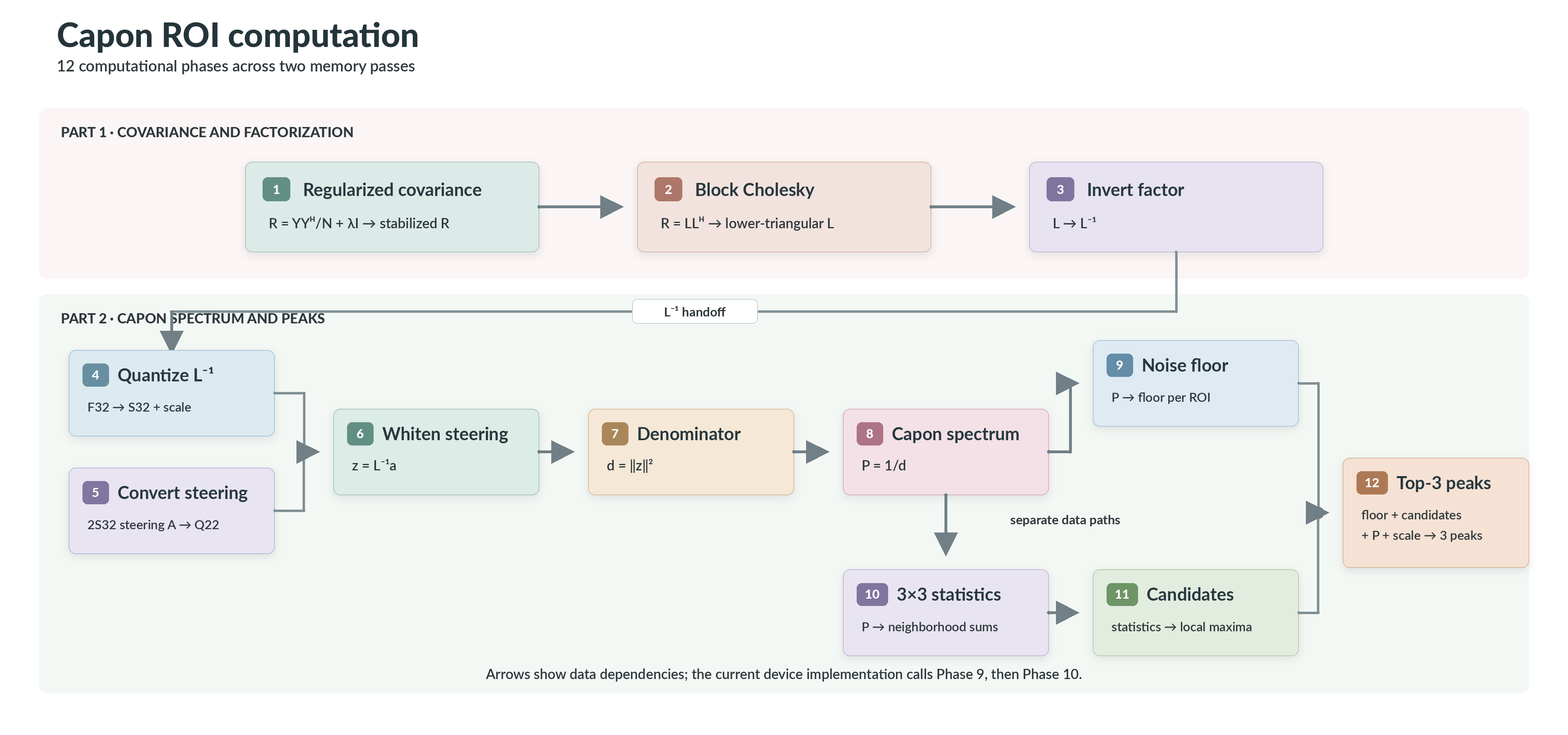
Figure 2: Capon ROI computation pipeline. The operator executes Phases 1 through 3 in Part 1 and Phases 4 through 12 in Part 2.#
Covariance and Regularization#
For each ROI, the sample covariance of the input snapshots is calculated as follows:
Here, \(\mathbf{Y}\in\mathbb{C}^{M\times N}\) is a slice of the Range-Doppler data cube for the range bin corresponding to the CFAR peak and for Doppler bins in a neighborhood around the CFAR peak’s Doppler bin, then projected into the ROI beamspace in the preprocessing stage. \(N\) is the configurable number of Doppler bins used to calculate the covariance matrix. \(M\) is the beamspace dimension, determined to be 16 for the current implementation as a tradeoff between performance and cost. \((\cdot)^H\) is the conjugate transpose. Because \(\mathbf{R} \in \mathbb{C}^{M\times M}\) is Hermitian, only its lower triangular elements are stored.
The covariance can be singular or poorly conditioned when snapshots are correlated. Then the FP32 Cholesky decomposition can fail. Adaptive diagonal loading regularizes it before factorization:
where \(\epsilon\) is the configurable adaptive loading constant. The loading shifts every covariance eigenvalue positively by a small amount, improving FP32 Cholesky robustness by preventing zero or negative eigenvalues.
Spectrum Evaluation#
The regularized covariance matrix is factored as
where \(\mathbf{L}\), called the Cholesky factor, is a lower-triangular matrix. We then compute the inverse of the Cholesky factor \(\mathbf{L}^{-1}\), which is also lower triangular. For each steering vector \(\mathbf{a}_k\), we compute the matrix-vector product:
The operator then evaluates the discrete Capon spectrum value for each steering vector without explicitly forming the inverse of the covariance matrix:
In practice, the matrix-vector product is grouped and implemented as a matrix-matrix product.
Peak Selection#
The Capon spectrum supplies two paths. One estimates the noise floor from the
lower median (64th-smallest of the 128 spectrum values). The other computes 3 x 3 neighborhood statistics and marks
prominent local maxima. Final ranking combines both paths: it keeps the three
strongest candidates and invalidates any candidate that does not strictly
exceed the estimated noise floor multiplied by a constant noiseFloorRatio. Equal candidate
values retain elevation-major grid order. Optional quadratic interpolation
then refines each accepted integer bin independently in azimuth and elevation
to obtain sub-bin accuracy.
Sub-bin Quadratic Interpolation#
When enableSubBinInterp is enabled, quadratic interpolation is
performed independently in azimuth and elevation. For the previous, center,
and next spectrum samples denoted as \(y_-\), \(y_0\), and
\(y_+\), respectively, the fitted quadratic is
The fractional offset is the vertex of this quadratic:
Each offset is accepted only when the center is strictly greater than both neighbors, the denominator is finite and nonzero, and \(|\delta|\leq 0.5\). Otherwise, that axis uses an offset of zero; failure on one axis does not disable a valid fit on the other. With interpolation disabled, the operator writes the integer argmax bin as an F32 value.
Configuration#
We provide 2 boolean configuration parameters:
useFpCovMatKnl: whether to use the FP32 covariance path or the S32 covariance path.enableSubBinInterp: whether to enable sub-bin interpolation.
Operator creation selects one of four embedded device executables from the
combination of useFpCovMatKnl and enableSubBinInterp.
For the useFpCovMatKnl option, input snapshots are always in 2S32 fixed-point format,
it is the covariance matrix calculation kernel that we choose to implement between FP32 and S32 intrinsics.
The S32 covariance path uses accelerated integer intrinsics and is preferred,
although intermediate truncation is required to avoid overflow.
When the input snapshot has a large dynamic range and lacks enough fractional bits,
the S32 path may not satisfy the final accuracy requirement. In that case, we should fall back to the FP32 path.
As for enableSubBinInterp, it is enabled by default.
We provide the option to turn it off because we found that, for some radar data,
sub-bin interpolation can harm accuracy when the azimuth-by-elevation search grid is fine and the underlying spectrum is not smooth.
The accuracy of operator depends on the underlying radar antenna layout and the choice of parameters. The algorithm choices are verified against the high-precision gold with the C reference (internal tooling), before the VPU implementation is compared with that reference.
Limitations#
We implement specialized kernels for the following fixed parameters, which we have verified on real data:
16-dimensional beamspace,
16 x 8 steering grid (16 azimuth points x 8 elevation points),
three output peaks per ROI (when fewer or no valid peaks are found, the operator marks each unused slot with
PVA_DOA_CAPON_ROI_INVALID_PEAK_POWER(-1.0f) inpeakPower),for the S32 covariance path, input snapshot Qbits must satisfy \(2Q_{\mathrm{input}}-\lfloor\log_2 N\rfloor > 16\), where \(N\) is the number of Doppler bins used to calculate the covariance matrix,
the remainder modulo 32 of the total number of Doppler bins used to calculate the covariance matrix, if nonzero, must be divisible by 4 and at least 12. This is to satisfy the VPU kernel unrolling requirements.
Sample Validation#
We provide a reference CPU implementation that mirrors the VPU implementation, with all floating-point values represented in FP32 and some computations using fixed-point arithmetic. We also provide 3 sets of golden data with different radar antenna layouts, where raw radar signals are simulated with MATLAB radar toolbox. The golden input data are prepared by running the radar pipeline up to before DoA and then the preprocessing stage. The golden output data are produced by fully FP64 reference Capon DoA pipelines in MATLAB or Python.
The radar_doa_capon_roi sample runs the operator on the capon_roi/16x16_ura dataset
(--assets <sample assets root>) and compares the VPU output with the fixed-point C reference.
We expect only numerical differences from FP32 operations here. The C reference itself is checked
against the MATLAB/Python high-precision gold by internal tooling.
MATLAB / Python high-precision gold
               |
               | internal reference-vs-gold check
               v
    CPU CREF algorithm mirror
               |
               | radar_doa_capon_roi
               v
          PVA VPU output
Device Implementation#
The implementation maps the algorithm in Figure 2 to two VPU memory passes within one command program. This section describes the arithmetic, block kernels, and data movement specific to that mapping.
Phase 2: Block Cholesky Decomposition#
Due to limited vector register capacity, we implement the Cholesky decomposition in a blockwise manner. The 16 x 16 complex Hermitian matrix is partitioned into 4 x 4 blocks. Elementwise Cholesky decomposition and inverse matrix computation are only done for the diagonal blocks, and all other blocks are just matrix multiplications. We combine the off-diagonal blocks in each pass for a deeper critical loop to improve kernel efficiency.
Since the covariance matrix is Hermitian, the diagonal elements are real. So for complex math, we only need multiplication and addition/subtraction operations, which are implemented with real math intrinsics.
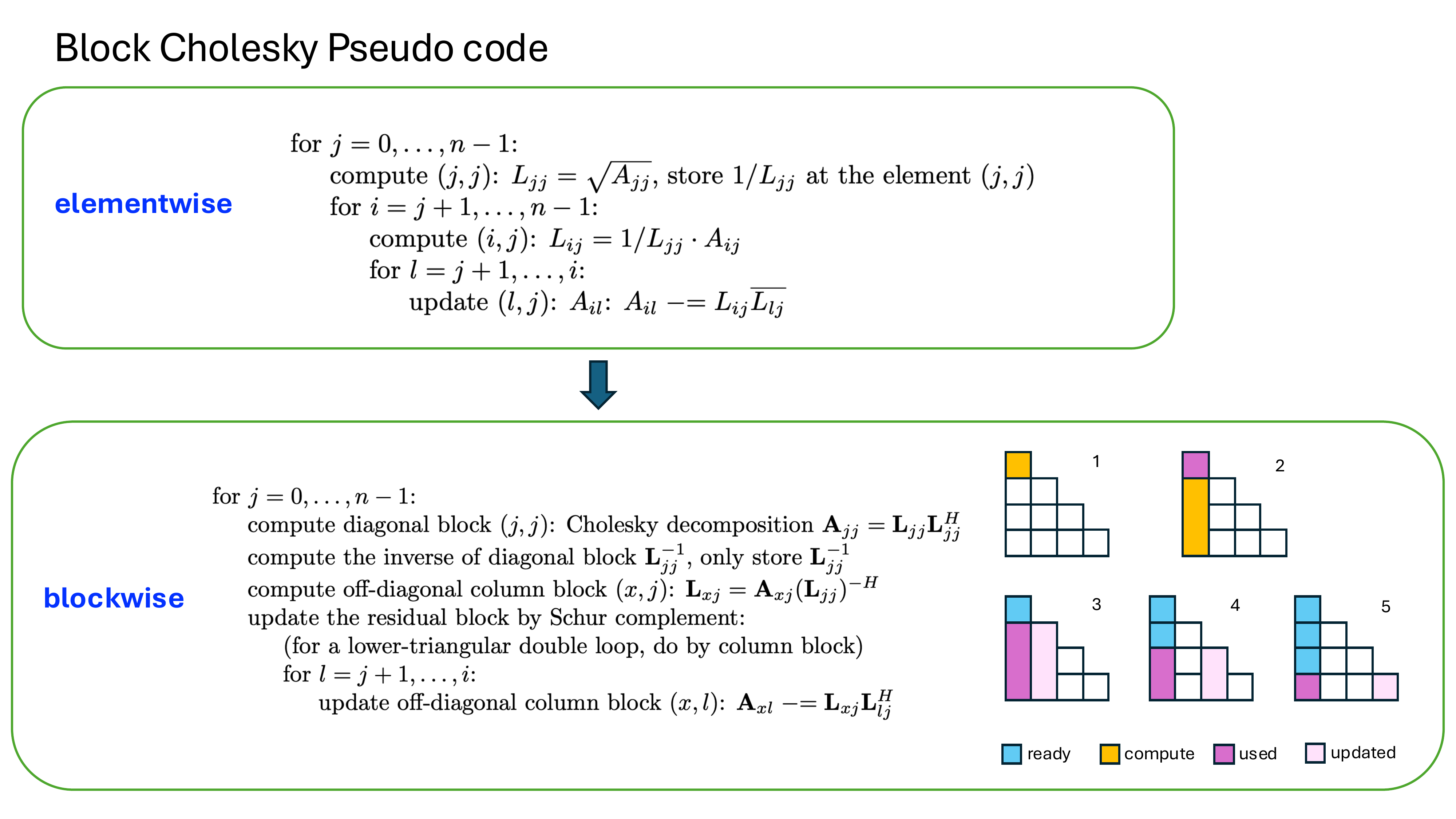
Figure 3: Block Cholesky schedule. Each numbered block becomes ready, is computed, is consumed by the below-diagonal solve, and updates the trailing matrix.#
Phase 3: Block Inverse of the Cholesky Factor#
The inverse of the Cholesky factor is computed by block forward substitution. After the block Cholesky decomposition, the diagonal blocks of the inverse of the Cholesky factor are already computed. Off-diagonal blocks are updated and computed as follows:
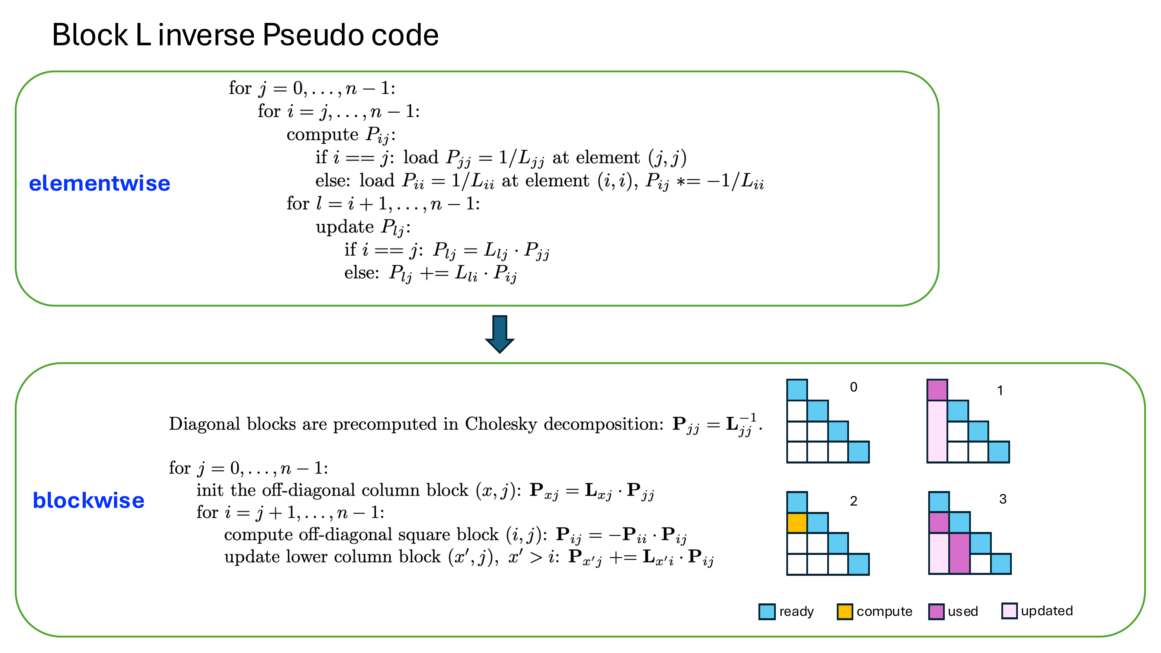
Figure 4: Block inverse schedule for the lower-triangular Cholesky factor. Previously completed blocks are accumulated before the next inverse block becomes available.#
Phases 4-5: Fixed-Point Quantization#
In Phase 4, Part 2 finds the maximum absolute element of the packed
\(\mathbf{L}^{-1}\) for each ROI. It scales the factor so that this maximum
maps to \(2^{28}\), then rounds the real and imaginary components to S32.
The per-ROI scale is retained so that Phase 12 can restore the reported FP32
power. In Phase 5, the steering vectors are converted from steeringQBits to
the internal Q22 format in place.
Phase 6: 8 x 8 Blocked Lower-Triangular Multiplication#
For each eight-ROI tile, the fixed-point product of the 16 x 16 inverse Cholesky factor and the steering vectors is computed with 8 x 8 blocks. Let \(\mathbf{B}=\mathbf{L}^{-1}\) and partition the matrix and each steering vector as
where \(\mathbf{B}_{00}\) and \(\mathbf{B}_{11}\) are 8 x 8 lower-triangular blocks, \(\mathbf{B}_{10}\) is a full 8 x 8 block, and each steering-vector half contains eight elements. The two output halves are
The implementation processes only the nonzero coefficients: 36 from each lower-triangular diagonal block and 64 from the full lower-left block, for 136 complex coefficients in total. The zero upper-right block requires no storage or arithmetic.
The VPU first computes the lower-right triangular product \(\mathbf{B}_{11}\mathbf{a}_{1,k}\), then accumulates the lower-left rectangular product \(\mathbf{B}_{10}\mathbf{a}_{0,k}\) into the same lower half. It computes the upper-left triangular product \(\mathbf{B}_{00}\mathbf{a}_{0,k}\) last. The operation overwrites the fixed-point steering-vector buffer in place with \(\mathbf{z}_k\). Before the rectangular accumulation, the lower-right result is clipped to \([-2^{30}, 2^{30}-1]\) to keep the following S48 accumulation in range.
Phases 7-8: Spectrum Evaluation#
In Phase 7, the VPU converts the fixed-point product to FP32 and accumulates \(\lVert\mathbf{L}^{-1}\mathbf{a}_k\rVert_2^2\) across the 16 beamspace dimensions. Phase 8 takes its reciprocal to form the FP32 Capon spectrum and creates a dynamically scaled U16 copy for peak selection.
Phases 9-12: Noise-Floor Estimation and Peak Selection#
The noise-floor path uses the ten most-significant bits of all 128 U16 spectrum values. Its result is the lower median, the 64th-smallest value, with the lowest six bits cleared. The current device schedule completes this path before it computes local-maximum statistics.
For every interior grid bin, let \(c\) be the center U16 value, \(m_{3\times3}\) its 3 x 3 maximum, and \(u\) the filter’s staged, integer-rounded approximation of the 3 x 3 sum divided by eight. The bin is a candidate when
The operator ranks candidates by descending U16 strength and keeps the first
three. A slot is valid only when its candidate value is strictly greater than
noiseFloorRatio times the noise-floor estimate. Invalid slots receive
PVA_DOA_CAPON_ROI_INVALID_PEAK_POWER (-1.0f) in peakPower; their azimuth
and elevation values are unspecified. Valid slots always have positive power,
and peakPower never contains NaN.
VPU I-cache Prefetch Strategy#
The total code size of the 1 command program with 2 memory passes greatly surpasses the 16 KB I-cache capacity of PVA. To prevent stalls from I-cache misses, we manually manage the instruction order and launch prefetch requests to pipeline I-cache prefetch latency with DMA data movement, ideally achieving zero I-cache-miss stalls on the VPU. The code sizes of both Part 1 and Part 2 are smaller than 16 KB, so we can place each stage in one cache window. Specifically, we add build control files (BCF) to align the code in execution order. We prefetch the Part 2 code when the Part 1 control code triggers the DMA write of the last tile.
On GEN3, we only do 1 prefetch as described above. However, on GEN2, we found that better performance can be achieved by 3 I-cache prefetches:
prefetch for part1 kernel functions at DMA read of the first snapshot tile,
prefetch for part2 control and initialization code after part1 control code triggers the DMA write of the last tile,
prefetch for part2 kernel functions at DMA read of the first intermediate value tile.
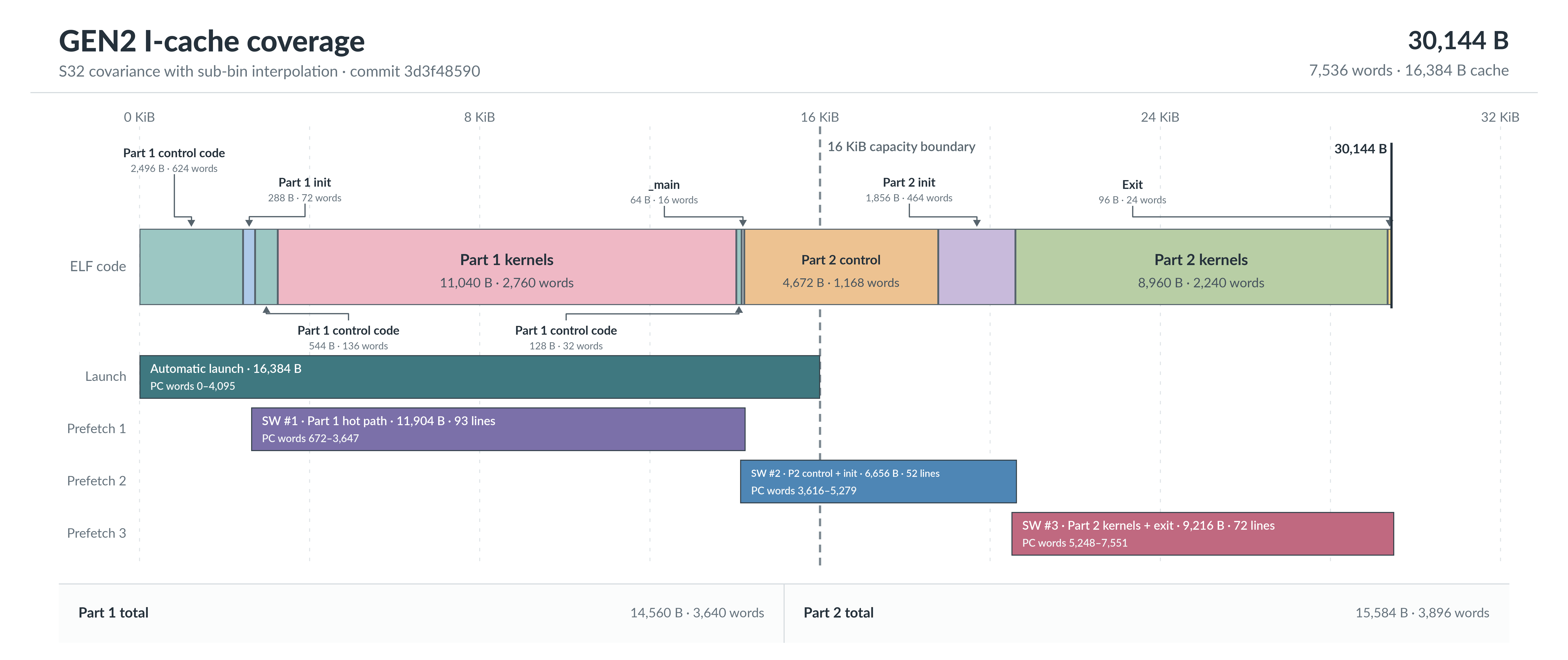
Figure 5: GEN2 code layout, automatic launch coverage, and three staged software I-cache prefetch requests.#
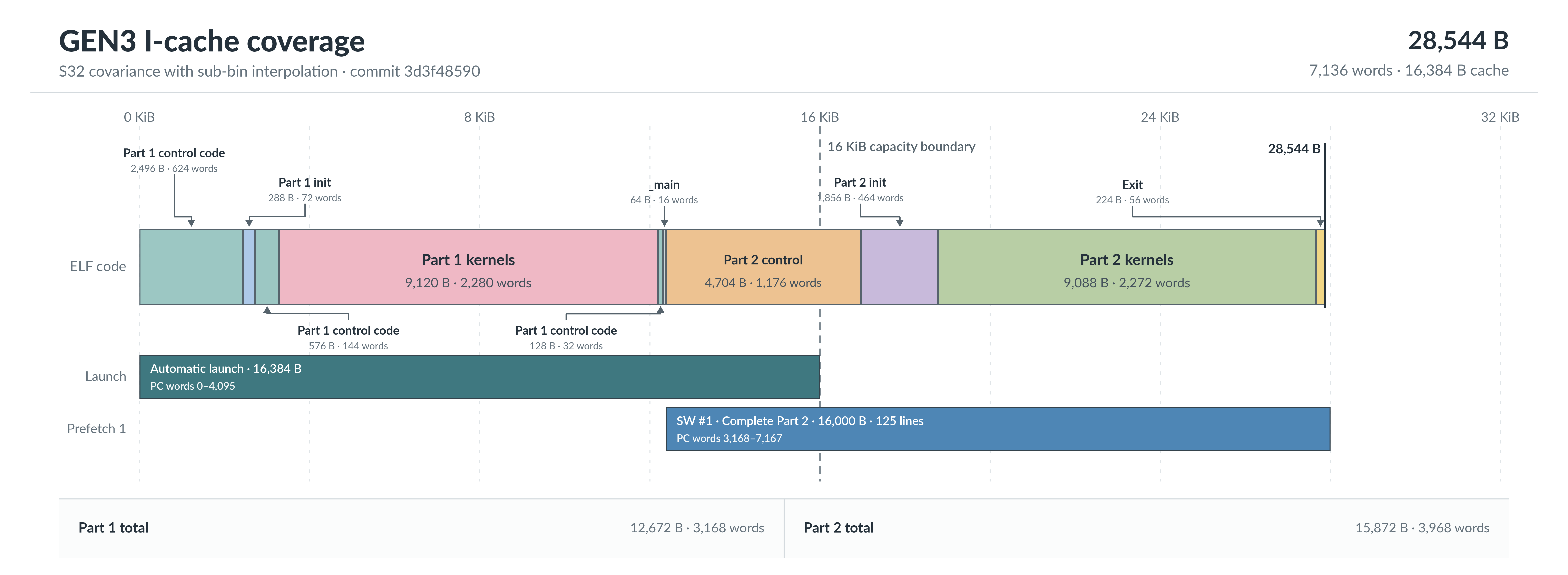
Figure 6: GEN3 code layout and the single software I-cache request covering the complete Part 2 phase.#
Synthetic Example: Capon vs Bartlett#
Figure 7 compares Capon with Bartlett on synthetic data: a single target and a pair 6° apart in azimuth, seen by a 16-element array (8 × 2, half-wavelength spacing) over 64 snapshots at about 20 dB SNR. Both references run on the same snapshots.
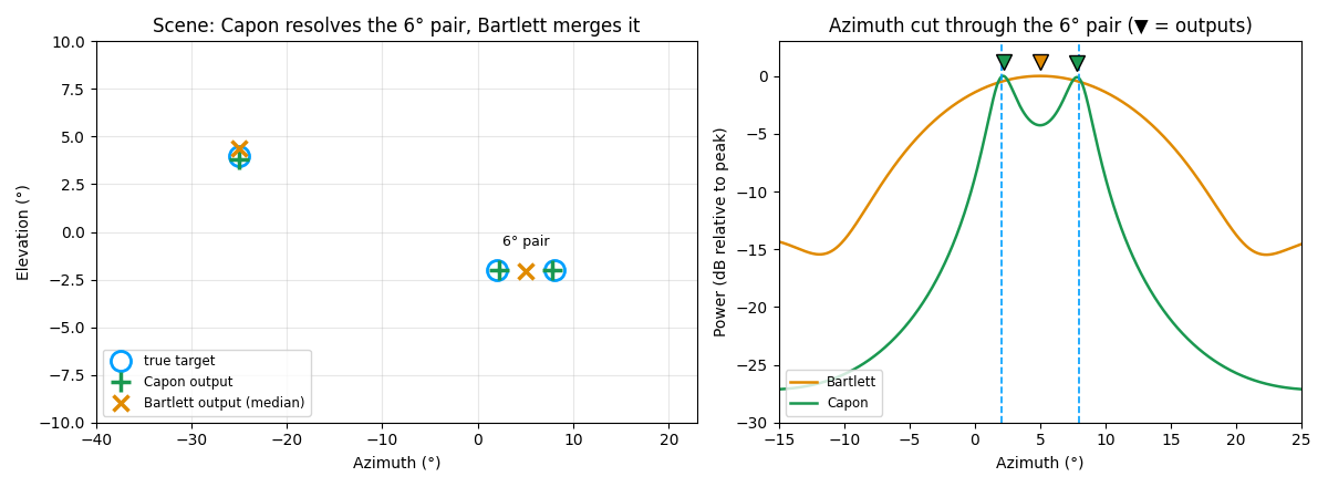
Figure 7: Left, true targets (○) and estimates: Capon (+) resolves the 6° pair, Bartlett (×) reports one angle between them. Right, an azimuth cut through the pair; the spectra are recomputed from the snapshots and the markers (▼) are the reference outputs.#
Performance#
Execution Time is the average time required to execute the operator on a single VPU core.
Note that each PVA contains two VPU cores, which can operate in parallel to process two streams simultaneously, or reduce execution time by approximately half by splitting the workload between the two cores.
Total Power represents the average total power consumed by the module when the operator is executed concurrently on both VPU cores.
Idle power is approximately 7.6 W on Jetson AGX Orin and 11.8 W on Jetson AGX Thor when the PVA is not processing data.
For detailed information on interpreting the performance table below and understanding the benchmarking setup, see Performance Benchmark.
Covariance Type |
ROIs |
Doppler Bins |
Execution Time |
Submit Latency |
Total Power |
|---|---|---|---|---|---|
S32 |
32 |
32 |
0.219ms |
0.004ms |
11.607W |
S32 |
32 |
64 |
0.263ms |
0.004ms |
11.607W |
S32 |
320 |
32 |
1.534ms |
0.004ms |
12.903W |
S32 |
320 |
64 |
1.981ms |
0.004ms |
12.903W |
S32 |
3200 |
32 |
14.680ms |
0.005ms |
13.302W |
S32 |
3200 |
64 |
19.126ms |
0.005ms |
13.701W |
F32 |
32 |
32 |
0.254ms |
0.004ms |
11.107W |
F32 |
32 |
64 |
0.337ms |
0.004ms |
11.006W |
F32 |
320 |
32 |
1.857ms |
0.004ms |
12.406W |
F32 |
320 |
64 |
2.672ms |
0.004ms |
11.506W |
F32 |
3200 |
32 |
17.867ms |
0.005ms |
12.803W |
F32 |
3200 |
64 |
26.011ms |
0.005ms |
12.304W |
Covariance Type |
ROIs |
Doppler Bins |
Execution Time |
Submit Latency |
Total Power |
|---|---|---|---|---|---|
S32 |
32 |
32 |
0.239ms |
0.003ms |
13.449W |
S32 |
32 |
64 |
0.290ms |
0.003ms |
13.854W |
S32 |
320 |
32 |
1.833ms |
0.003ms |
14.349W |
S32 |
320 |
64 |
2.307ms |
0.003ms |
14.45W |
S32 |
3200 |
32 |
17.762ms |
0.003ms |
14.743W |
S32 |
3200 |
64 |
22.800ms |
0.003ms |
15.239W |
F32 |
32 |
32 |
0.324ms |
0.003ms |
13.651W |
F32 |
32 |
64 |
0.437ms |
0.003ms |
13.155W |
F32 |
320 |
32 |
2.573ms |
0.003ms |
13.752W |
F32 |
320 |
64 |
3.848ms |
0.003ms |
13.651W |
F32 |
3200 |
32 |
25.265ms |
0.003ms |
14.54W |
F32 |
3200 |
64 |
38.091ms |
0.003ms |
14.045W |
References#
C. Waldschmidt, C. Bonfert, and T. Grebner, Millimeter Wave Radar: Hardware and Signal Processing, 1st ed. Cham: Springer, 2025, ch. 7, “Methods for Angle Estimation,” pp. 133-142. doi:10.1007/978-3-031-89118-2_7.