

HistogramEqualization#
Overview#
Histogram Equalization is an image processing technique used to enhance the contrast of images by effectively spreading out the most frequent intensity values in an image, i.e., stretching out the intensity range of the image. The method is particularly effective when the usable data of the image is represented by close contrast values.
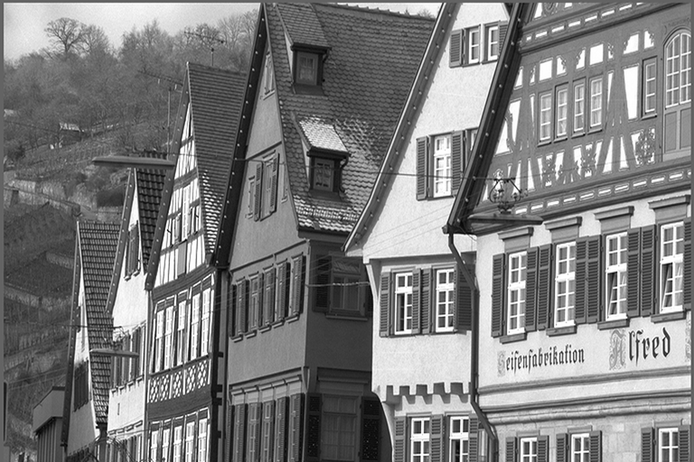
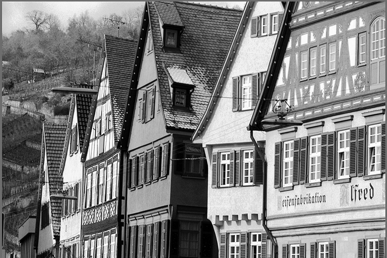
The following example demonstrates the effect of histogram equalization on a grayscale image:
Input Image |
Output Image |
|---|---|
|
|
As shown in the example above, histogram equalization significantly improves the visual quality by redistributing the intensity values across the full dynamic range, making previously hidden details more visible and enhancing overall image contrast.
Algorithm Description#
This algorithm aims to find a new mapping palette based on the histogram. Consider a grayscale image X, whose total number of gray levels in the image is L (\(L=256\) for 8-bit images). Denote the histogram of the image as \(H_x\).
Classical Histogram Equalization Theory#
The theoretical foundation follows these steps:
Probability Distribution: The probability of occurrence of a pixel of level i in the image is:
\[p[i] = \frac{H_x[i]}{N}\]where \(N\) is total number of pixels in the image
Cumulative Distribution Function (CDF): The cumulative distribution function corresponding to \(p[i]\) is:
\[\operatorname{cdf}_x[i] = \sum_{j=0}^{i} p[j]\]Intensity Transformation: Using the cumulative distribution function to transform the original pixel value to a new pixel value:
\[y[i] = \operatorname{cdf}_x[i] \times (L - 1)\]
Practical Implementation Considerations#
The actual implementation modifies the classical algorithm for robustness and performance:
Direct Histogram Computation: Calculate frequency counts directly without probability conversion:
\[H_x[i] = \text{count of pixels with intensity } i\]Cumulative Histogram: Compute cumulative sums using integer arithmetic:
\[\operatorname{CDF}[i] = \sum_{j=0}^{i} H_x[j]\]Fixed-Point Implementation: The VPU implementation uses fixed-point arithmetic (with 15-bit precision) for optimal performance. Once the histogram is complete, four device kernels run in sequence: the cumulative sum, the minimum-value search, the lookup-table build, and its replication across the lookup ways.
Minimum Value Detection and Cumulative Distribution:
The algorithm first finds the minimum non-zero cumulative value to prevent contrast compression and computes the full cumulative distribution:
\[\operatorname{CDF}_{\min} = \min\{\operatorname{CDF}[i] : \operatorname{CDF}[i] > 0\}\]Mathematical Transformation:
The robust intensity transformation applies normalized transformation that handles edge cases:
\[y[i] = \frac{\operatorname{CDF}[i] - \operatorname{CDF}_{\min}}{(M \times N) - \operatorname{CDF}_{\min}} \times 255\]where \(M \times N\) is the total number of pixels in the image.
Fixed-Point Arithmetic with 15-bit Precision:
The core transformation uses fixed-point arithmetic to maintain precision while optimizing for VPU performance as below:
\[\begin{split}\text{scale} &= \frac{255 \times 2^{15}}{(M \times N) - \operatorname{CDF}_{\min}} \\[0.7em]\end{split}\]\[\begin{split}\quad\operatorname{normalized\_CDF} &= \operatorname{CDF}[i] - \operatorname{CDF}_{\min} \\[0.7em]\end{split}\]\[\begin{split}\quad\text{y}[i] &= \left\lfloor\frac{\operatorname{normalized\_CDF} \times \text{scale}}{2^{15}}\right\rfloor \\\end{split}\]Key Implementation Benefits:
Numerical Stability: Avoids division by zero when all pixels have the same intensity
Integer Arithmetic: Eliminates floating-point operations for VPU efficiency
Proper Contrast Stretching: \(\operatorname{CDF}_{\min}\) normalization maps the lowest occupied intensity to 0
Fixed-Point Precision: 15-bit scaling; the scale is truncated, so the brightest output can fall short of 255 (253 for a 1920 x 1080 image)
Vectorized Pixel Transformation: The final step applies the pre-computed lookup table to transform input pixels using vectorized lookup operations for optimal performance.
Parameters#
Input data type: u8 (8-bit unsigned)
Input format: Single-channel grayscale image
Output data type: u8 (8-bit unsigned)
Data Layout: HWC (Height x Width x Channels)
Implementation Details#
Dataflow Configuration#
The implementation uses three RasterDataFlow (RDF) configurations for efficient data movement and processing:
Source RDF:
Essential for histogram computation phase
Configured with input dimensions and tile size (\(TW \times TH\))
Second Source RDF:
Uses same input dimensions and shares the tile buffer of the first source RDF
Essential in histogram equalization phase for pixel remapping
Destination RDF:
Configured with same tile dimensions as input
Each RDF is configured with a tile shape chosen at Create to cover the image in the fewest tiles and uses double buffering to overlap computation and data transfer.
Buffer Allocation#
The implementation requires several VMEM buffers:
One double-buffered input tile buffer, shared by the histogram and apply passes
Histogram buffer (\(256\) bins \(\times 32\) vector width)
Normalized histogram buffer (\(256\) bins)
Output buffer for transformed image tiles
Additional buffers for intermediate computations
Kernel Implementation and Vectorization#
The operator makes two passes over the image: the first accumulates the histogram, the second maps every pixel through the finished table. Seven device kernels run in this order:
knl_hist— count the tile’s active samples into the 32-way halfword histogramknl_drain— fold the 32 ways of each bin into the 32-bit counts, then clear the waysknl_scan— inclusive cumulative counts across the 256 binsknl_delta— \(\text{delta} = \min\{\text{accum}[i] : \text{accum}[i] > 0\}\)knl_lut— \(\text{lut}[i] = (\max(\text{accum}[i] - \text{delta},\ 0) \times \text{scale}) \gg 15\)knl_replicate— broadcast each table entry across its 32 lookup waysknl_apply— \(\text{dst} = \text{lut32}[\text{src}]\), 32 pixels per lookup
knl_hist and knl_apply are the hot stages, each bound at one M0 issue per 32 pixels. The
scan, minimum, table and replication kernels run over 256 bins once per frame, so their cost does not scale with image size; the drain also works on 256 bins but runs every HEQ_DRAIN_ISSUES issues.
Counting (knl_hist). One vhist_simple_32h issue handles 32 pixels, one per
sub-histogram, so updates within an issue cannot collide. It takes the histogram pointer, a vector
of pixel values serving as bin indices, and a per-lane weight supplied as the row mask. The mask
doubles as the update vector — a zero-weight lane is a no-op — so columns past the image width need
no predication; interior tile columns are passed an all-ones mask and only the last column carries a
real one. A short final tile row is handled by shortening the issue count instead. The loop is
split into a chess_unroll_loop(8) part and a short remainder, because rounding the trip count up
would inject counts no later stage could subtract.
Folding (knl_drain). The 32 ways of a bin are contiguous in one 64-byte line, so each bin
costs a single vector load. vsumr_s reduces each half of that line and the two scalar results are
added, giving the bin’s total for this drain; that total is added to the bin’s running 32-bit count
and the halfword ways are cleared. This runs whenever the issues since the last drain reach
HEQ_DRAIN_ISSUES, and once more after the last tile: each issue adds one to a single bin per way,
so draining before that count reaches the signed 16-bit limit is what keeps the halfword bins from
overflowing.
Cumulative sum (knl_scan). Hillis-Steele doubling, eight passes. The shifted operand is taken
at an address offset rather than a lane permute, so each pass is one load pair plus one add. Both
cumulative buffers carry a leading pad of zero words so the shifted read always lands on real zeros,
and the pass count is even, so the result ends up back in the primary buffer.
Minimum (knl_delta). Every bin below the lowest occupied intensity is empty, so that bin’s
cumulative value equals its raw count and is the smallest positive value in the array — which turns a
first-nonzero search into a min-reduce. Empty bins are parked at 0x7FFFFFFF with dvmux so they
cannot win, the array is reduced with dvmin, and vminr_s collapses the two halves. An empty
histogram returns zero.
Normalization (knl_lut). Delta is subtracted from each cumulative value and the result clamped
at zero: bins below the lowest occupied intensity must come out zero, and re-deriving them with the
final delta would give a negative numerator that the reference’s uint16_t cast wraps into a large
value. dvmulw then applies the scale, followed by an explicit 15-bit right shift since no
truncating mode is available for word multiplies. The scale is
\(\frac{255 \times 2^{15}}{(width \times height) - delta}\), matching the reference’s integer
division; a constant image makes delta equal the sample count, so the divisor is clamped to at least
one. The product stays at or below \(255 \times 2^{15}\), inside the 48-bit lane.
Replication (knl_replicate). Lane i of the parallel lookup reads only sub-table i, so the
logical table must be present in all 32. Entry b of way i sits at byte \(2i + 64b\) — one
64-byte line per bin, exactly one vector store. This replicated table, not the dense one, is what the
apply pass indexes.
Applying the table (knl_apply). vlookup_32hu performs 32 simultaneous lookups per issue,
taking the replicated table pointer and a vector of pixels as indices. Each iteration loads 32
pixels, applies the table, clamps at 255 and stores. There is no weight mask and no predication: the
output RasterDataFlow transfers only the columns and rows inside the image, so a group running past
the valid width writes tile-buffer bytes the DMA never reads. As in the histogram pass the loop is
unrolled by eight with a short remainder.
The implementation optimizes performance through:
Vector histogram instructions for parallel bin updates
Address generators for efficient memory access patterns
Double buffering for overlapped data transfer and computation
A tile shape chosen at Create to cover the image in the fewest tiles
Vector reduction operations for histogram computation
Performance#
Execution Time is the average time required to execute the operator on a single VPU core.
Note that each PVA contains two VPU cores, which can operate in parallel to process two streams simultaneously, or reduce execution time by approximately half by splitting the workload between the two cores.
Total Power represents the average total power consumed by the module when the operator is executed concurrently on both VPU cores.
Idle power is approximately 7.6 W on Jetson AGX Orin and 11.8 W on Jetson AGX Thor when the PVA is not processing data.
For detailed information on interpreting the performance table below and understanding the benchmarking setup, see Performance Benchmark.
Image Size |
Data Type |
Execution Time |
Submit Latency |
Total Power |
|---|---|---|---|---|
1280x720 |
U8 |
0.131ms |
0.003ms |
14.529W |
1920x1080 |
U8 |
0.270ms |
0.004ms |
14.726W |
Image Size |
Data Type |
Execution Time |
Submit Latency |
Total Power |
|---|---|---|---|---|
1280x720 |
U8 |
0.091ms |
0.002ms |
18.041W |
1920x1080 |
U8 |
0.177ms |
0.003ms |
18.132W |