

DepthToSpace#
Overview#
DepthToSpace squeezes the depth dimension and moves the squeezed elements into both the width and height dimensions. Depth here is synonymous with the channel dimension, and these terms are used interchangeably. The total number of elements remains the same, and the output width and height are both enlarged by a ratio known as the block size. The reverse operation is called SpaceToDepth. Unless explicitly stated otherwise, the channel, height and width refer to the input dimensions in this document.
Reference Implementation#
The operation follows the ONNX definition in DCR (depth-column-row) ordering. Given an input of shape \([C, H, W]\) and block size \(B\), the output has shape \([C / B^2, H \cdot B, W \cdot B]\), and every output element is:
where:
\(C\), \(H\) and \(W\) refer to the input channel, height and width.
\(B\) refers to the block size, and \(C\) is a multiple of \(B^2\).
\(c\) refers to the output channel, and \(h\) and \(w\) to the input row and column.
\(bx\) and \(by\) refer to the position within a block, with \(0 \le bx, by < B\).
Values are copied unmodified, and every input element appears exactly once in the output. More information can be found in [1].
TensorFlow’s depth_to_space API is used as the reference code to generate the golden output. In the following code snippet, both “input” and “output” are TensorFlow tensors in NCHW layout.
import tensorflow as tf
output = tf.nn.depth_to_space(input, block_size=blocksize, data_format="NCHW")
The same API also generates the mapping table that the gather/scatter path permutes through. That table is the operation applied to a \([B^2, tileY, tileX]\) tensor holding an iota sequence [2] of uint16_t type. TensorFlow cannot be called at runtime within the PVA solutions, so the table is built there with the NVCV API instead, as described in Mapping Table Calculation.
Implementation Details#
The operator carries two device implementations of the same rearrangement, and the choice between them is made at create time. The raster path runs when its dataflows can express the shape, and the gather/scatter path runs otherwise. Both produce the same output, and either supports the full parameter range below.
Limitations#
The supported ranges of the DepthToSpace parameters are listed as following, and a shape outside them is rejected at create time, naming the single property that is out of range:
The block size is 2, 3 or 4.
The data type is
uint8_torint8_t.The input tensor has rank 3 and CHW layout, and its channel count is a multiple of \(B^2\).
The input tensor may carry padding, but its regions must not overlap. Elements within a row are contiguous, the row stride is at least the width, and the channel stride is at least the height times the row stride.
Every extent and stride is positive and below \(2^{31}\), and so is the channel count times the channel stride, because the transfers address the tensor through 32-bit offsets.
The row stride is at most 65535, the width of the 16-bit surface line pitch.
\(W \cdot B\) and \(H \cdot B\) are each at most 65535, the widths of the 16-bit output surface fields.
The output tensor is derived from the input tensor and the block size, and is tightly packed.
Dataflow Configuration#
This section and the two that follow describe the gather/scatter path, whose source is named depthtospace_gsdf_top.c. It places no requirement on the tensor layout, so it serves every shape the operator accepts.
1 input GatherScatterDataFlow(GSDF), 1 output GSDF and 1 RasterDataFlow(RDF) are needed,
1 input GSDF is used to gather the \(B^2\) input tiles that make one output tile from DRAM into a ping-pong buffer in VMEM.
1 output GSDF is used to transfer the output tile from a ping-pong buffer in VMEM to DRAM.
1 RDF is used to transfer the mapping table from DRAM to VMEM one time.
On the second PVA generation the input tiles are spread over up to four GSDF handlers, chosen by block size, and later generations use a single handler. Every tile address is an explicit linear offset accumulated from the row stride and the channel stride, so this path carries any padding the operator accepts. Its tile grid is built from the prime factorization of the extents, so every tile is whole and no DMA padding is needed.
The tile grid divides the input height and width into \((H / tileY) \cdot (W / tileX)\) pieces, and the channel dimension into \(C / B^2\) pieces. An input tile holds \(B^2 \cdot tileY \cdot tileX\) elements, and the output tile it produces is \((tileY \cdot B) \cdot (tileX \cdot B)\). The following figure gives a simple example, where \(C = 8\), \(H = 2\), \(W = 2\), \(B = 2\), \(tileX = 1\) and \(tileY = 1\). Each colored square represents an element.
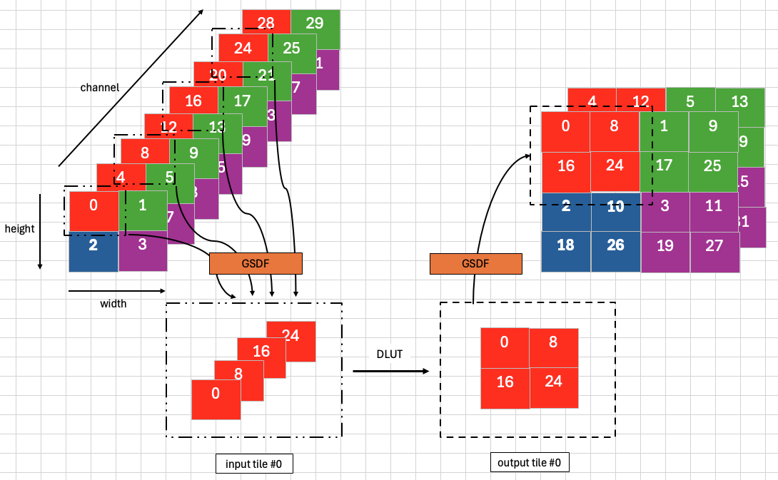
Figure 1: Tiling Example of 1x8x2x2 Input with Block Size = 2#
Larger tiles perform better, as the control overhead is about the same per transfer. The tile size is determined at create time, in three steps:
If the whole tensor fits the tile budget, no tiling is needed and the tile is the whole image.
Otherwise, if the width, height and block size match one of the pre-calculated cases, the pre-calculated tile size is used.
Otherwise the width and the height are factored into primes, and every combination that draws from both is a candidate \(\{tileX, tileY\}\) pair. Candidates above the tile budget are discarded, and the largest of the rest is selected, breaking a tie on the larger \(tileX\).
Profiling on silicon is still needed for manual checking, as there is no cycle-accurate model to evaluate performance in native mode. When the width or the height is a large prime number, the enumeration leaves \(tileX = tileY = 1\), which still runs but performs poorly.
Buffer Allocation#
3 VMEM buffers are needed,
1 DLUT input buffer with ping-pong buffering for the input tiles.
1 DLUT output buffer with ping-pong buffering for the output tiles.
1 buffer for the mapping table.
The device declares a 120 KiB scratch arena on each of the three superbanks, and the host places the three buffers within them. Ping-pong buffering leaves 60 KiB for one tile, which is the tiling constraint:
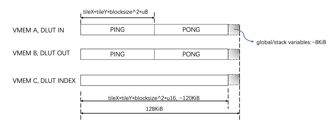
Figure 2: VMEM Allocations#
Kernel Implementation#
The kernel permutes each tile with the DLUT in 1D lookup mode. The DLUT handles memory bank conflicts itself, and a table calculated beforehand lets it permute the input in an arbitrary pattern.
It operates on a chunk of elements per call, so the input is divided into tiles that the dataflows move in step with it. The DLUT index entries are uint16_t, so one call addresses at most 65536 elements.
Mapping Table Calculation#
If \(tileX = tileY = 1\), the mapping table is an iota sequence starting from zero. Otherwise NVCV APIs generate it, in the same steps as the reference code:
Construct an
NVCVTensorDataobject of shape {B, B, 1, tileY, tileX}, holding anNVCVTensorBufferobject filled with an iota sequence ofuint16_ttype.Construct an
NVCVTensorLayoutobject with the layout to be permuted as {1, tileY, B, tileX, B}.Permute that layout object and the strides within the buffer object with
nvcvTensorShapePermute, in two calls, as no NVCV API permutes shape and strides at once.Traverse the elements of the buffer object using the permuted shape and strides, in the way PyTorch’s contiguous function traverses a tensor. The traversed sequence is the mapping table.
Raster Path#
The raster path carries the rearrangement in the surface declarations and the address generators. Its sources are named depthtospace_rdf_top.c and depthtospace_rdf_knl.c.
Three terms are used throughout this section:
- Flattened input row index \(r\)
\(r = c \cdot H + h\), the row index a channel group’s \(C / B^2\) channels take once they are viewed as one raster. A group is therefore \((C / B^2) \cdot H\) rows of \(W\) bytes.
- Channel group \(g\)
\(g = by \cdot B + bx\), the \(C / B^2\) input channels that share one base offset. There are \(B^2\) of them.
- Output row offset \(by\)
One of the \(B\) programs the operation is split into. Row offset \(by\) owns the output rows \(r \cdot B + by\), that is every \(B\)-th row starting at \(by\). Note this is unrelated to the phase label
CmdProgram::addDataFlowHeadtakes, which the operator never sets.
The following figure follows the same example as Figure 1, where \(C = 8\), \(H = 2\), \(W = 2\) and \(B = 2\). Each square is one element, labelled with its index in the input, and coloured by the channel group it belongs to.
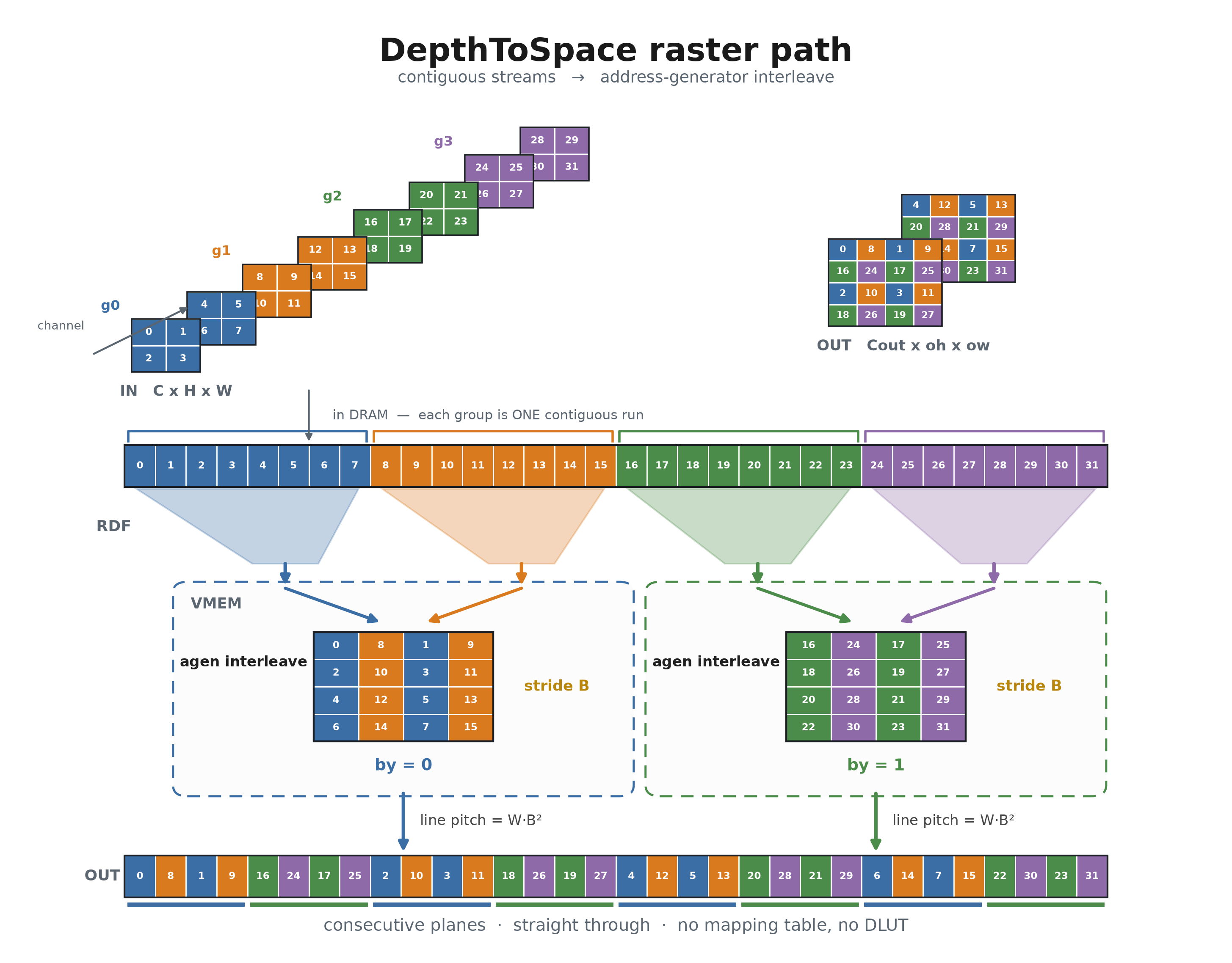
Figure 3: Raster Path Data Flow for 1x8x2x2 Input with Block Size = 2#
Row offset \(by\) reads the \(B\) channel groups \(by \cdot B + bx\) and writes the output rows \(r \cdot B + by\). It is its own program, of \(B\) input RasterDataFlows and one output RasterDataFlow, and the \(B\) programs are submitted in a single CupvaStreamSubmit. The \(B\) groups it reads share one \((W \times (C / B^2) \cdot H)\) geometry and differ only by a fixed base offset, so they alias onto one handler.
The output flow’s line pitch is \(W \cdot B^2\), which makes the rows of row offset \(by\) the rows of a plain raster based at \(by \cdot W \cdot B\). In the figure, \(W = 2\) and \(B = 2\) give a pitch of 8 and a base of 4 for \(by = 1\). Selecting every \(B\)-th output row is therefore the output flow’s job, and the kernel fills a dense tile.
Three properties of those dataflows bound the shapes the path can describe:
At most 256 tiles per raster dimension, which caps the flattened row count at 8192.
An output line pitch of at most 65535, that is \(W \cdot B^2 \le 65535\). This is stricter than the operator’s own output width limit of \(W \cdot B \le 65535\), and a shape between the two runs on the gather/scatter path.
A channel stride the flattened raster can express, which holds when a channel group carries a single channel or the channel stride is exactly the height times the row stride.
Each block size gets its own device executable, built with BLK_SZ fixed, so the tile geometry and the address generator strides are compile-time constants. The input tile is the largest multiple of 32 columns that keeps the output tile at or below 256 columns: 128 x 32 for block size 2, and 64 x 32 for block sizes 3 and 4. The tile height is 32, because a transposed byte access moves 32 lanes of one row each. Buffers are the \(B\) input tiles, one per channel group, and the output tile. All are double-buffered and declared with TRANS_MODE_1, which pads the VMEM line pitch to the value a transposed byte access requires. The input tiles alternate across superbanks A and B by \(bx\), so the \(B\) loads issue in parallel. The output tile and the scalars sit on superbank C, which therefore sees only writes.
The kernel loop performs no vector-ALU operation at all: its body is \(B\) transposed loads and \(B\) transposed stores, so the memory slots are its only floor. The interleave is the element stride of the store address generator, which is \(B\), since no vector store writes a strided pattern and the instruction set has no three-way interleaving store.
Each \(bx\) gets its own destination generator, because a generator advances after every access and \(B\) stores through one generator would step \(B^2\) bytes per iteration. The base of destination generator \(bx\) is offset by \(bx\), so stream \(bx\) lands on byte \(bx\) of every output column group.
The source generators walk the columns of the tile, each access loading one column across 32 rows. A transposed byte access requires a transpose line pitch of the form \(64 \cdot k + 2\), which TRANS_MODE_1 guarantees. The lane offset \(k\) is derived from the VMEM tile line pitch the kernel reads back from the dataflow handler.
Why the Raster Path Exists#
The operator does not expose the choice of data flow: a shape either satisfies the three raster constraints above and runs the raster path, or it runs the gather/scatter path. The table below is what that choice is worth, on the four shapes the KPI suite profiles, all of which either path can serve.
Input Tensor Shape |
Block Size |
Execution Time, raster |
Execution Time, gather/scatter |
Speedup |
|---|---|---|---|---|
4 x 128 x 128 |
2 |
0.049±0.003ms |
0.054±0.005ms |
1.11x |
4 x 1024 x 1024 |
2 |
0.451±0.010ms |
0.771±0.036ms |
1.71x |
36 x 368 x 640 |
3 |
0.896±0.027ms |
2.025±0.042ms |
2.26x |
16 x 2048 x 2048 |
4 |
6.719±0.071ms |
16.468±0.032ms |
2.45x |
Execution Time carries the same meaning as in the benchmark tables below: the mean over 128 submits, plus or minus three standard deviations, of the operator on a single VPU core including internal task scheduling overhead. Measured on AGX Orin with PVA SDK 2.9.4. Both columns come from one binary on one board, the gather/scatter column produced by forcing that path for shapes the selection rule would otherwise route to the raster path, so the two differ only in the data flow.
The smallest shape is the exception that shows what is being measured. Its raster kernel occupies the VPU for 12us against the gather/scatter path’s 31us, a ratio of 2.6, but a fixed submit overhead of roughly 37us sits on both and flattens the column above to 1.11. The ratio the other three rows show is the one that survives once the workload is larger than the overhead.
The gap has a single cause. The gather/scatter path spends VPU cycles on the permutation itself: it runs the DLUT over every tile, and the table that drives the DLUT must be built and transferred before the first tile moves. The raster path expresses the same rearrangement in the load and store address generators, so its inner loop issues \(B\) loads and \(B\) stores and nothing else, and no table exists. The ratio is therefore roughly flat in the input size rather than growing with it.
Performance#
Execution Time is the average time required to execute the operator on a single VPU core.
Note that each PVA contains two VPU cores, which can operate in parallel to process two streams simultaneously, or reduce execution time by approximately half by splitting the workload between the two cores.
Total Power represents the average total power consumed by the module when the operator is executed concurrently on both VPU cores.
Idle power is approximately 7.6 W on Jetson AGX Orin and 11.8 W on Jetson AGX Thor when the PVA is not processing data.
For detailed information on interpreting the performance table below and understanding the benchmarking setup, see Performance Benchmark.
Input Shape (CHW) |
Data Type |
Block Size |
Execution Time |
Submit Latency |
Total Power |
|---|---|---|---|---|---|
4x128x128 |
U8 |
2 |
0.043ms |
0.003ms |
9.311W |
4x1024x1024 |
U8 |
2 |
0.359ms |
0.004ms |
15.629W |
36x368x640 |
U8 |
3 |
0.705ms |
0.008ms |
15.931W |
16x2048x2048 |
U8 |
4 |
4.744ms |
0.009ms |
16.746W |
Input Shape (CHW) |
Data Type |
Block Size |
Execution Time |
Submit Latency |
Total Power |
|---|---|---|---|---|---|
4x128x128 |
U8 |
2 |
0.045ms |
0.002ms |
13.256W |
4x1024x1024 |
U8 |
2 |
0.396ms |
0.003ms |
16.25W |
36x368x640 |
U8 |
3 |
0.745ms |
0.004ms |
20.3W |
16x2048x2048 |
U8 |
4 |
4.304ms |
0.010ms |
22.589W |