

MedianFilter#
Overview#
The median filter performs a two-dimensional (2D) filtering operation on the input image by replacing each pixel with the median value within the neighborhood defined by the 2D kernel [1].
Unlike linear filters like Gaussian blur or mean filter, the median filter preserves sharp edges while effectively removing noise, making it particularly valuable for various image processing applications. By replacing each pixel with the median value from its neighborhood rather than the mean, it’s much less sensitive to extreme values (outliers) than linear techniques.
Common applications of the median filter include impulse noise reduction, image smoothing, and pre-processing for computer vision algorithms.
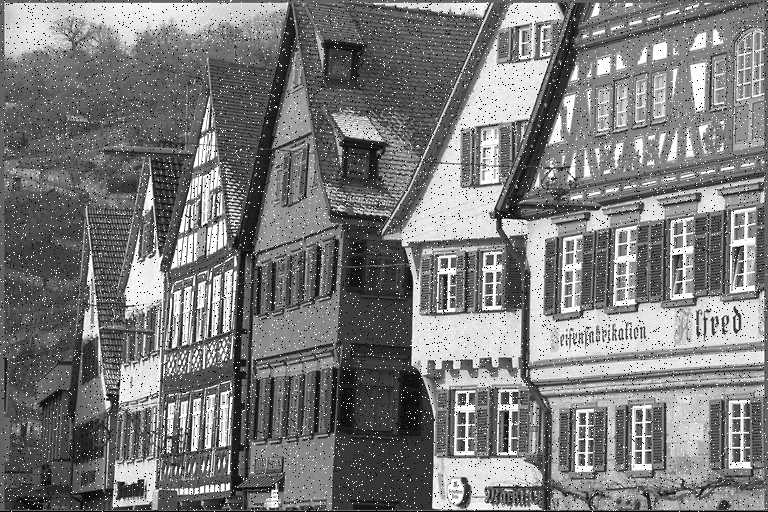
Input Image (5% salt-and-pepper noise) |
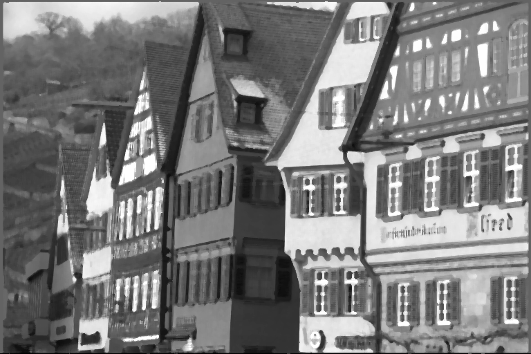
Output Image |
|---|---|
|
|
MedianFilter Parameters: kernel size = 5×5, replicate border.
Implementation#
In the current implementation, two border handling methods are supported: zero padding and clamp (border pixel extension). All supported image formats are: U8, Y8, Y8_ER, S8, U16, Y16, Y16_ER, S16, 2S16, U32 and S32.
We only support taking median of all elements in the kernel window; this corresponds to the box kernel
type in VPI [1]. All kernel sizes (3x3, 5x5, 5x7, and 7x7) are supported for all image formats.
Data Flow Configuration#
RasterDataFlow (RDF) is used for both input and output data flows.
The input RDF is configured with halo and circular buffer, to fetch pixels outside the tile and reuse overlapping pixels between tiles.
The output RDF is configured with ping-pong buffer, to parallelize the DMA and VPU workloads.
Tile sizes are chosen to maximize DMA read/write bandwidth. The total tile size is fixed at 16 KB: each tile is 128 scalars of type \(\text{T}\) wide and \(128/\text{sizeof(T)}\) rows tall, where \(\text{T}\) is the data type of one image channel. In terms of pixels, the 2S16 format carries 2 interleaved channels, so its tiles are 64 pixels wide; all other formats are single-channel, so their tiles are 128 pixels wide. With these dimensions, the tile width in bytes is a multiple of 64 B and the fixed 16 KB tile size achieves full ADB/VDB efficiency. A width of 128 scalars is also divisible by the vector length of every supported data type, so vector instructions in the VPU kernels run at maximal parallelism.
When the input image size is not exactly a multiple of the tile size, RDF will automatically add padding to the last row/column tiles up to a full tile, and kernel functions will run on the padded tiles. Then the output data flow will only move out pixels within the valid region of the output image.
Border Handling#
The two supported border types can be directly realized by the two padding modes in RDF:
zero: PAD_CONST, padding by constant with value 0
clamp: PAD_BPE, padding by border pixel extension (BPE)
For input image format 2S16, simply applying padding by BPE will only copy the outer channel value, instead of padding the boundary pixel into channel-interleaved pattern as desired. To tackle this issue, the input RDF is configured with data type int32_t, regarding the 2 interleaved channels as a single int32_t value. Then padding by BPE results into correct channel-interleaved border values.
Kernel Processing#
The median filter is implemented by a two-pass approach. For each input tile, the passes iterate through kernel windows of all output pixels in the tile:
1st pass: sort row elements in each kernel window and store temporary sorted values. Duplicate rows are only sorted once.
2nd pass: combine the presorted rows and find the median value for each output pixel.
For 3x3 kernels, a specialized implementation is used to find the median. All larger kernels (5x5, 5x7, and 7x7) process a 2x2 neighborhood of output pixels together so that overlapping regions can share sorting work; for channel-interleaved 2S16 the tile is first split into two single-channel planes (see below). This routing is selected automatically from the image format and kernel size; it does not require an API option.
3x3 Kernel Size#
In the 1st pass, the 3 elements in each row are sorted. The minimum, middle and maximum values of the 3 elements are obtained by instructions vmin3/vmid3/vmax3.
In the 2nd pass, the median value turns out to be the middle value of 3 elements (middle is obtained by vmid3):
maximum of the minimum values in each row (obtained by vmax3)
minimum of the maximum values in each row (obtained by vmin3)
middle of the middle values in each row (obtained by vmid3)
Separable Sorting Network with 2x2 Reuse#
To further accelerate the median filter, the implementation applies the separable sorting network with 2x2 reuse described in [2] to all 5x5, 5x7, and 7x7 kernels. Four adjacent output pixels are processed together as a 2x2 group. Because their kernel windows overlap substantially, each shared region is sorted once and reused by every kernel window that contains it.
The implementation uses two passes. For a kernel with \(m\) rows and \(n\) columns, the four kernel windows span \(m + 1\) rows by \(n + 1\) columns. In the first pass, we sort the central \(n - 1\) elements of all \(m + 1\) rows in the union footprint. For the 5x5 example, this is the highlighted strip comprising four columns and six rows. The row-presort operation advances horizontally with a stride of 2, matching the 2x2 output grouping. The row presorts are small odd-even sorting networks; Figure 1 illustrates the construction for a row of five elements.
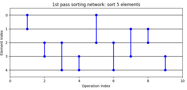
Figure 1: Row sorting network (5-element example). Horizontal lines carry the row elements; each vertical connector is one compare-exchange operation.#
In the second pass, we combine the presorted rows with the remaining elements of each kernel window as follows:
Merge the \(m - 1\) presorted rows in the shared core, each of length \(n - 1\), and keep the middle \(m + n\) elements.
Separately merge the result from step a with each presorted extra row (upper and lower). Each row contains \(n - 1\) elements; keep the middle \(m + 1\) elements from each merged result.
Sort the left and right extra columns separately, each of length \(m - 1\).
Merge each result from step b with each sorted column from step c to form the four output branches, and keep the middle two elements from each merged result.
Merge each result from step d with its corner element to obtain the corresponding median.
Figure 2 shows the actual second-pass sorting network of one kernel window for the 5x5 kernel, following the stages above.
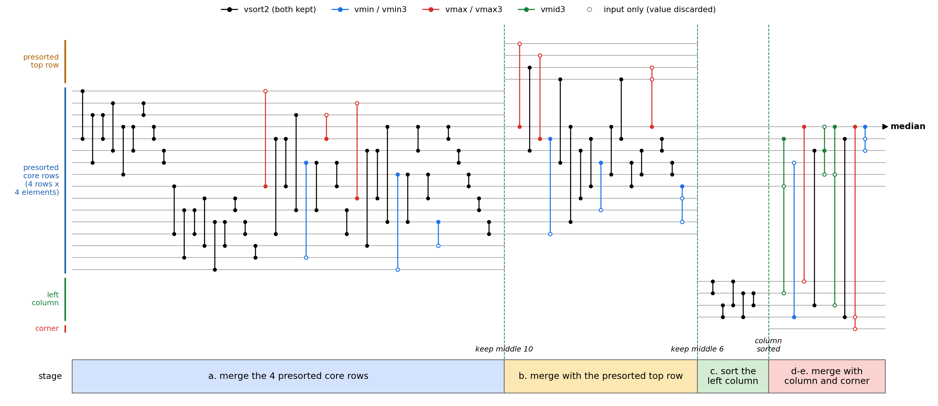
Figure 2: Second-pass sorting network for one kernel window (top-left) of a 2x2 output group with a 5x5
kernel, as implemented. Horizontal lines carry the window’s elements; each vertical connector is one
operation: black vsort2 keeps both outputs, while for the colored single-output operations the filled
dot marks the produced value and open circles mark inputs whose value is discarded. Lines ending at a
stage boundary are pruned — they can no longer affect the median.#
At each merge stage, we retain only values that can still become the median and prune the sorting network accordingly. As explained in [2], the number of kept elements in each stage is determined by a fact that when a sorted list containing at least \(k + 1\) elements is combined with \(k\) additional elements, only the middle \(k + 1\) elements of the current list can affect the median of the combined list.
The pruning also shapes the operation mix. First, a vsort2 whose upper or lower output port is dead
regresses to a single-output compare: vmin when only the low value is kept, or vmax when only the high
value is kept. The pruned network is then regrouped into three-input comparators where possible: consecutive
vmin (vmax) operations fold into vmin3 (vmax3); a vmax result feeding only a vmin (or
vice versa), and a vsort2 whose two outputs feed exactly one vmax and one vmin, fold into vmid3
(median-of-3). Each candidate fold is validated before use: the vmin3/vmax3 folds are exact on every
wire, while the vmid3 folds may change intermediate values that were only partially pruned, so they are
proven by exhaustive 0-1 enumeration of the composed two-pass selection network — the retained ranks of every
stage, and therefore the final median, remain bit-exact. Among the validated foldings, each kernel keeps the
combination with the best measured performance: folding removes operations, but the VLIW schedule determines
the loop’s initiation interval, so a fold is adopted only when the measured schedule improves.
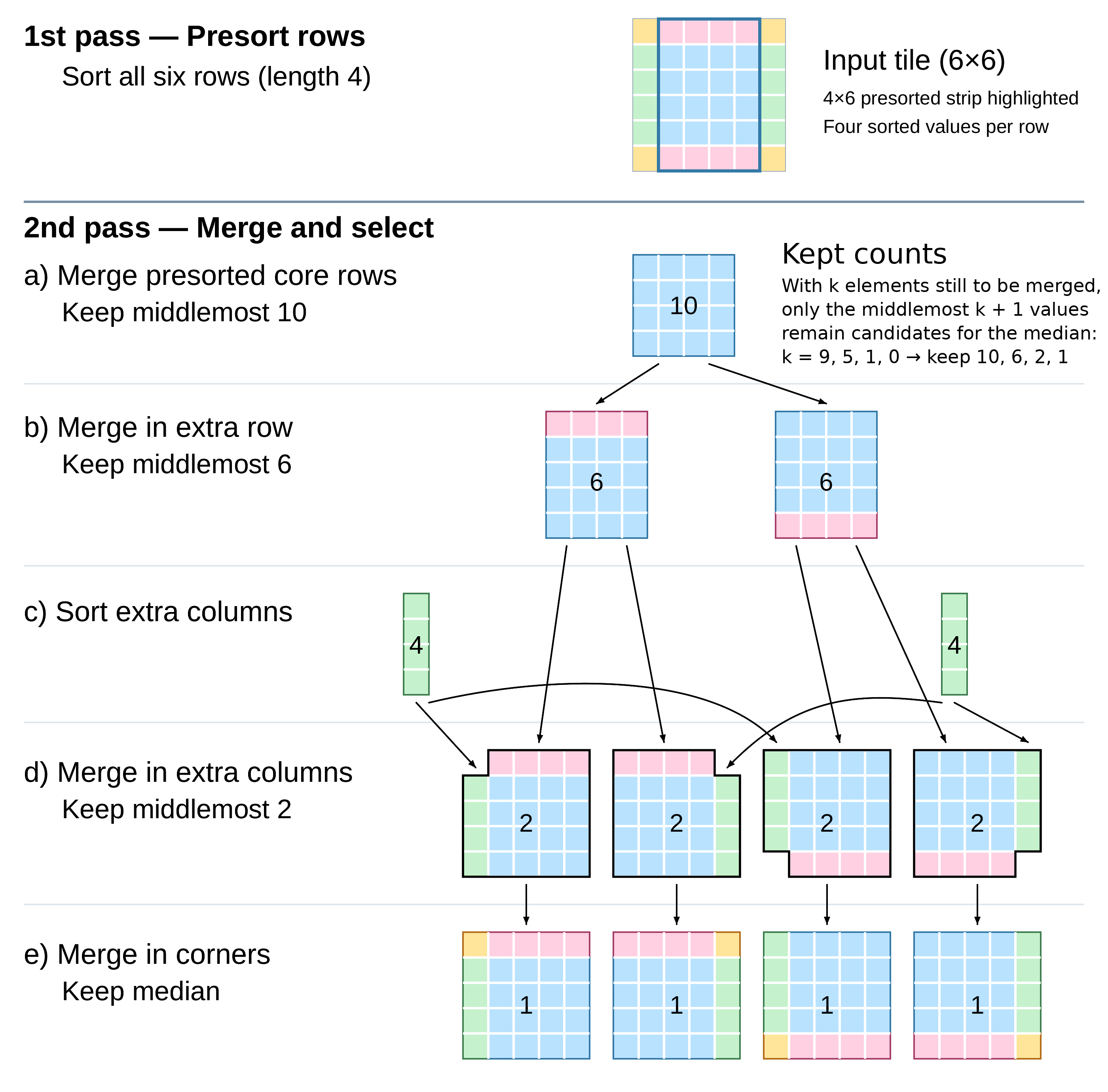
Figure 3: Two-pass computation of a 2x2 output group for a 5x5 median filter.#
2S16 Input#
For channel-interleaved 2S16 input, the 3x3 kernel loads the input with deinterleaving double-vector loads of agen stride 2, separating the two channels into the low and high parts of the double vectors; both channels are processed together by the double-vector min/mid/max operations and re-interleaved by the store.
The 5x5, 5x7, and 7x7 kernels use the separable sorting network with 2x2 reuse. The 2x2 scheme obtains its even/odd-pixel split from the stride-2 deinterleaving double-vector loads, but for channel-interleaved data that deinterleave level is consumed by the channel split. Instead of doubling the register pressure of the sorting loops, each tile is first deinterleaved into two flat single-channel planes by a small memory-bound copy loop, the unmodified single-channel separable pipeline runs once per plane, and a second small copy loop re-interleaves the two planar outputs into the destination tile. The copy overhead is a few percent of the tile; the sorting work is identical to two single-channel S16 tiles. The 5x5 and 5x7 programs also use taller tiles than the single-channel programs to amortize per-tile overhead over the half-width per-channel planes; the 7x7 program keeps the default tile height, which its larger halo and intermediate buffers already fill the vector memory with.
Performance#
Execution Time is the average time required to execute the operator on a single VPU core.
Note that each PVA contains two VPU cores, which can operate in parallel to process two streams simultaneously, or reduce execution time by approximately half by splitting the workload between the two cores.
Total Power represents the average total power consumed by the module when the operator is executed concurrently on both VPU cores.
Idle power is approximately 7.6 W on Jetson AGX Orin and 11.8 W on Jetson AGX Thor when the PVA is not processing data.
For detailed information on interpreting the performance table below and understanding the benchmarking setup, see Performance Benchmark.
Image Size |
Kernel Size |
Image Format |
Execution Time |
Submit Latency |
Total Power |
|---|---|---|---|---|---|
1920x1080 |
3x3 |
U8 |
0.294ms |
0.004ms |
15.019W |
1920x1080 |
3x3 |
S8 |
0.294ms |
0.004ms |
15.817W |
1920x1080 |
3x3 |
U16 |
0.537ms |
0.005ms |
15.418W |
1920x1080 |
3x3 |
S16 |
0.537ms |
0.005ms |
15.817W |
1920x1080 |
3x3 |
2S16 |
1.182ms |
0.006ms |
15.716W |
1920x1080 |
3x3 |
U32 |
1.060ms |
0.006ms |
15.317W |
1920x1080 |
3x3 |
S32 |
1.061ms |
0.005ms |
15.716W |
1920x1080 |
5x5 |
U8 |
1.720ms |
0.004ms |
11.006W |
1920x1080 |
5x5 |
S8 |
1.719ms |
0.004ms |
11.405W |
1920x1080 |
5x5 |
U16 |
3.278ms |
0.006ms |
11.006W |
1920x1080 |
5x5 |
S16 |
3.279ms |
0.006ms |
11.405W |
1920x1080 |
5x5 |
2S16 |
7.400ms |
0.006ms |
11.405W |
1920x1080 |
5x5 |
U32 |
6.505ms |
0.006ms |
11.005W |
1920x1080 |
5x5 |
S32 |
6.503ms |
0.006ms |
11.404W |
1920x1080 |
5x7 |
U8 |
1.778ms |
0.004ms |
11.405W |
1920x1080 |
5x7 |
S8 |
1.778ms |
0.004ms |
11.804W |
1920x1080 |
5x7 |
U16 |
3.348ms |
0.005ms |
11.405W |
1920x1080 |
5x7 |
S16 |
3.348ms |
0.006ms |
12.203W |
1920x1080 |
5x7 |
2S16 |
7.487ms |
0.006ms |
11.804W |
1920x1080 |
5x7 |
U32 |
6.721ms |
0.007ms |
11.405W |
1920x1080 |
5x7 |
S32 |
6.723ms |
0.006ms |
11.804W |
1920x1080 |
7x7 |
U8 |
2.638ms |
0.004ms |
11.305W |
1920x1080 |
7x7 |
S8 |
2.638ms |
0.004ms |
11.704W |
1920x1080 |
7x7 |
U16 |
4.980ms |
0.006ms |
11.305W |
1920x1080 |
7x7 |
S16 |
4.982ms |
0.006ms |
11.704W |
1920x1080 |
7x7 |
2S16 |
10.790ms |
0.005ms |
11.704W |
1920x1080 |
7x7 |
U32 |
10.011ms |
0.004ms |
11.305W |
1920x1080 |
7x7 |
S32 |
10.013ms |
0.006ms |
11.704W |
Image Size |
Kernel Size |
Image Format |
Execution Time |
Submit Latency |
Total Power |
|---|---|---|---|---|---|
1920x1080 |
3x3 |
U8 |
0.331ms |
0.003ms |
17.061W |
1920x1080 |
3x3 |
S8 |
0.331ms |
0.003ms |
17.468W |
1920x1080 |
3x3 |
U16 |
0.604ms |
0.003ms |
17.468W |
1920x1080 |
3x3 |
S16 |
0.603ms |
0.003ms |
17.456W |
1920x1080 |
3x3 |
2S16 |
1.332ms |
0.004ms |
16.858W |
1920x1080 |
3x3 |
U32 |
1.195ms |
0.004ms |
17.253W |
1920x1080 |
3x3 |
S32 |
1.195ms |
0.003ms |
17.265W |
1920x1080 |
5x5 |
U8 |
1.932ms |
0.003ms |
13.854W |
1920x1080 |
5x5 |
S8 |
1.932ms |
0.003ms |
13.854W |
1920x1080 |
5x5 |
U16 |
3.687ms |
0.003ms |
13.854W |
1920x1080 |
5x5 |
S16 |
3.687ms |
0.003ms |
13.854W |
1920x1080 |
5x5 |
2S16 |
8.317ms |
0.003ms |
13.854W |
1920x1080 |
5x5 |
U32 |
7.321ms |
0.004ms |
13.752W |
1920x1080 |
5x5 |
S32 |
7.321ms |
0.003ms |
13.752W |
1920x1080 |
5x7 |
U8 |
2.001ms |
0.003ms |
13.854W |
1920x1080 |
5x7 |
S8 |
2.001ms |
0.003ms |
13.854W |
1920x1080 |
5x7 |
U16 |
3.770ms |
0.003ms |
13.854W |
1920x1080 |
5x7 |
S16 |
3.771ms |
0.003ms |
13.854W |
1920x1080 |
5x7 |
2S16 |
8.414ms |
0.003ms |
13.752W |
1920x1080 |
5x7 |
U32 |
7.575ms |
0.003ms |
13.752W |
1920x1080 |
5x7 |
S32 |
7.574ms |
0.003ms |
14.146W |
1920x1080 |
7x7 |
U8 |
2.970ms |
0.003ms |
13.752W |
1920x1080 |
7x7 |
S8 |
2.970ms |
0.003ms |
13.752W |
1920x1080 |
7x7 |
U16 |
5.610ms |
0.003ms |
13.55W |
1920x1080 |
7x7 |
S16 |
5.610ms |
0.003ms |
13.651W |
1920x1080 |
7x7 |
2S16 |
12.147ms |
0.003ms |
13.752W |
1920x1080 |
7x7 |
U32 |
11.281ms |
0.003ms |
13.651W |
1920x1080 |
7x7 |
S32 |
11.281ms |
0.003ms |
13.752W |