Channel Estimation for Uplink Shared Channel (PUSCH) in pyAerial

This notebook provides researchers an example of how to prototype machine learning in pyAerial. PyAerial is the Python bindings for the Aerial SDK, NVIDIA’s L1 and L2 accelerated stack that is also integrated in the Aerial Omniverse Digital Twin (AODT). This enables researchers to develop standard-compliant approaches focusing on enhancing their link-level performance. Subsequently, the approach can be evaluated realistically in AODT, showing how the link-level performance translates to system-level KPIs.

In particular, this notebook focuses on improving the channel estimation based on the DMRS pilots in a PUSCH transmission. First, we isolate the channel estimator block from the pyAerial PUSCH pipeline. The channel estimation is on one of the first receiver blocks, as seen in the figure below:

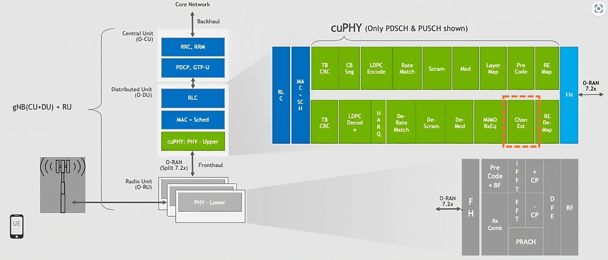
To isolate the channel estimation block, we refer to the modular PUSCH pipeline in Example PUSCH Simulation.ipynb. There, we see how to interface channel estimation downstream with resource element (RE) demapper and with the wireless channel, and upstream with other components like the MIMO Equalizer. Similar approaches can be done for other blocks in the receiver or transmitter pipelines.

This notebook uses PyTorch to train a convolutional neural network that improves and interpolates least squares (LS) channel estimates. The training uses a custom LS estimator which interfaces with a resource grid, resource mapper, and channel generator from Sionna. The trained models are then integrated and validated in pyAerial PUSCH pipeline with standard-compliant signal transmission and reception blocks running on top of Sionna channels.

*

            

            
[1]:
        

            

            
import os
# GPU setup
GPU_IDX = 2
os.environ["CUDA_VISIBLE_DEVICES"] = str(GPU_IDX)  # Select only one GPU
os.environ['TF_CPP_MIN_LOG_LEVEL'] = "3"  # Silence TensorFlow.

import torch
import numpy as np
from tqdm import tqdm
import tensorflow as tf
import matplotlib.pyplot as plt

# Our imports
from channel_gen_funcs import SionnaChannelGenerator
from channel_gen_funcs import PyAerialChannelEstimateGenerator
from channel_est_models import ChannelEstimator
from channel_est_models import ComplexMSELoss
import utils as ut

dev = torch.device(f'cuda')
torch.set_default_device(dev)

# General parameters
num_prbs = 48               # Number of PRBs in the UE allocated bandwidth
interp = 1                  # Interpolation factor. If 2, it estimates also for REs without DMRS
models_folder = f'saved_models_prbs={num_prbs}_interp={interp}' # Folder to save trained models

# Training parameters
train_snrs = np.array([10]) # Train models for these SNRs. Suggested: np.arange(-10, 40.1, 10)
training_ch_model = 'UMa'   # Channel model ['Rayleigh', 'CDL-x', 'TDL-x', 'UMa', 'UMi'],
                            # where x is in ["A", "B", "C", "D", "E"] as per TR 38.901
n_iter = 5000               # Number of training iterations. Best results: 30k
batch_size = 32             # Batch size = number of channels to train simultaneously
model_reuse = True          # Whether to load the weights of the last trained model
                            # (this trick improves convergence speed considerably)

# Testing parameters
test_snrs = np.arange(-10, 40.1, 5)  # Test models for these SNRs. Suggested: np.arange(-10, 40.1, 5)
testing_ch_model = 'UMi'             # Channel for testing
n_iter_test = 1000                   # Number of batches of channels to evaluate (batch=32)
        

            

            
[PhysicalDevice(name='/physical_device:GPU:0', device_type='GPU')]
        

The example machine learning model uses the least squares (LS) estimates and outputs a more accurate channel estimate. In its base configuration, the DMRS has 1/2 density in frequency (i.e. one RE for every two subcarriers). Therefore, our ChannelEstimator can either output as many estimates as DMRS pilots (half of the subcarriers using an interpolation factor interp=1) or twice as many estimates (with the parameter interp=2) thus covering all subcarriers.

Important note on training: Our approach consists of training one model per SNR. SNR-specific models can learn more accurately how to estimate the channels for SNRs close to the original SNR that was used for model training. This approach also solves the problem where low SNR channels incur in higher loss and lead to the model focusing on them and not working for the high SNR cases.

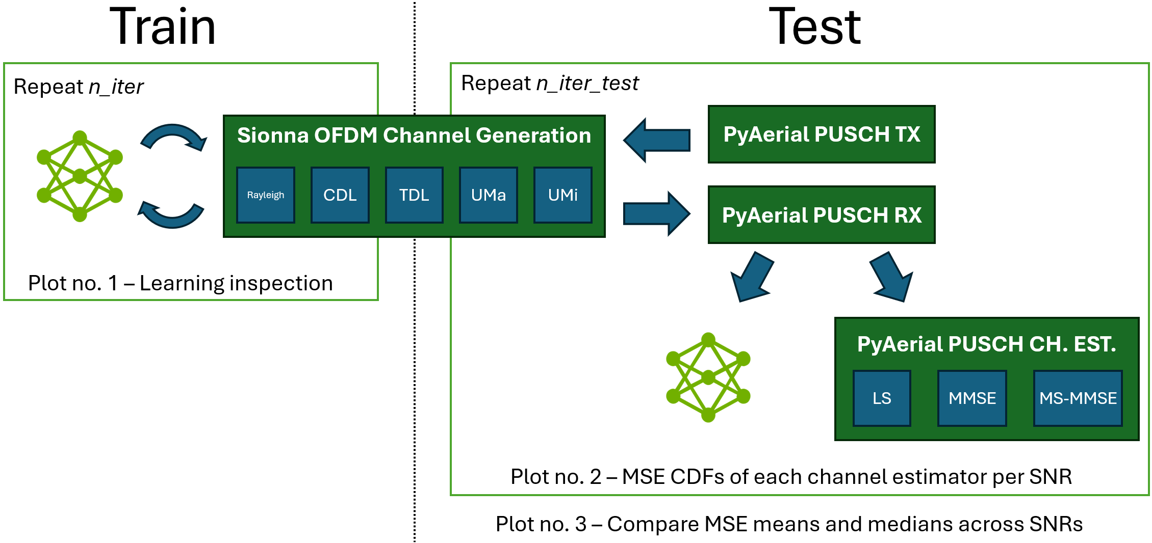
For training, the model interfaces directly with Sionna channel models. For testing, the model is integrated in pyAerial’s PUSCH pipeline and evaluated alongside other classic channel estimators, like the minimum mean squared error (MMSE) and the multi-stage MMSE (MS-MMSE). A diagram of training and testing is below:

            

            
[2]:
        

            

            
models_dir = ut.get_model_training_dir(models_folder, training_ch_model,
                                       num_prbs, n_iter, batch_size)
os.makedirs(models_dir, exist_ok=True)

# Channel generator for training
train_ch_gen = SionnaChannelGenerator(num_prbs, training_ch_model, batch_size)

last_model = ''
for snr_idx, snr in enumerate(train_snrs):
    print(f'Training model for SNRs:{snr}dB')
    save_model_path = ut.get_snr_model_path(models_dir, snr)

    model = ChannelEstimator(num_prbs*12//2, freq_interp_factor=interp).to(dev)
    reload_last_model = model_reuse and last_model
    if reload_last_model:
        model.load_state_dict(torch.load(last_model))

    criterion = ComplexMSELoss()
    optimizer = torch.optim.AdamW(model.parameters(), lr=1e-3, weight_decay=1e-4)

    model.train()
    train_loss, mse_loss = [], []
    count = []
    for i in (pbar := tqdm(range(n_iter // (5 if reload_last_model else 1)))):
        h, h_ls = train_ch_gen.gen_channel_jit(snr)

        # Transition tensors to PyTorch for learning
        h, h_ls = torch.tensor(h.numpy()).to(dev), torch.tensor(h_ls.numpy()).to(dev)

        # Uncomment to inspect estimates vs ground-truth channel
        # ut.compare_ch_ests([h_ls.cpu().numpy()[0,:], h.cpu().numpy()[0,:]],
        # ['LS', 'GT'], title=f'SNR = {snr} dB')

        h_hat = model(h_ls[..., ::2])

        loss = criterion(h_hat, h[..., ::(3-interp)])
        optimizer.zero_grad(); loss.backward(); optimizer.step()

        train_loss += [ut.db(loss.item())]
        pbar.set_description(f"Iteration{i+1}/{n_iter}")
        pbar.set_postfix_str(f"Training loss:{train_loss[-1]:.1f}dB")

    last_model = save_model_path
    torch.save(model.state_dict(), save_model_path)
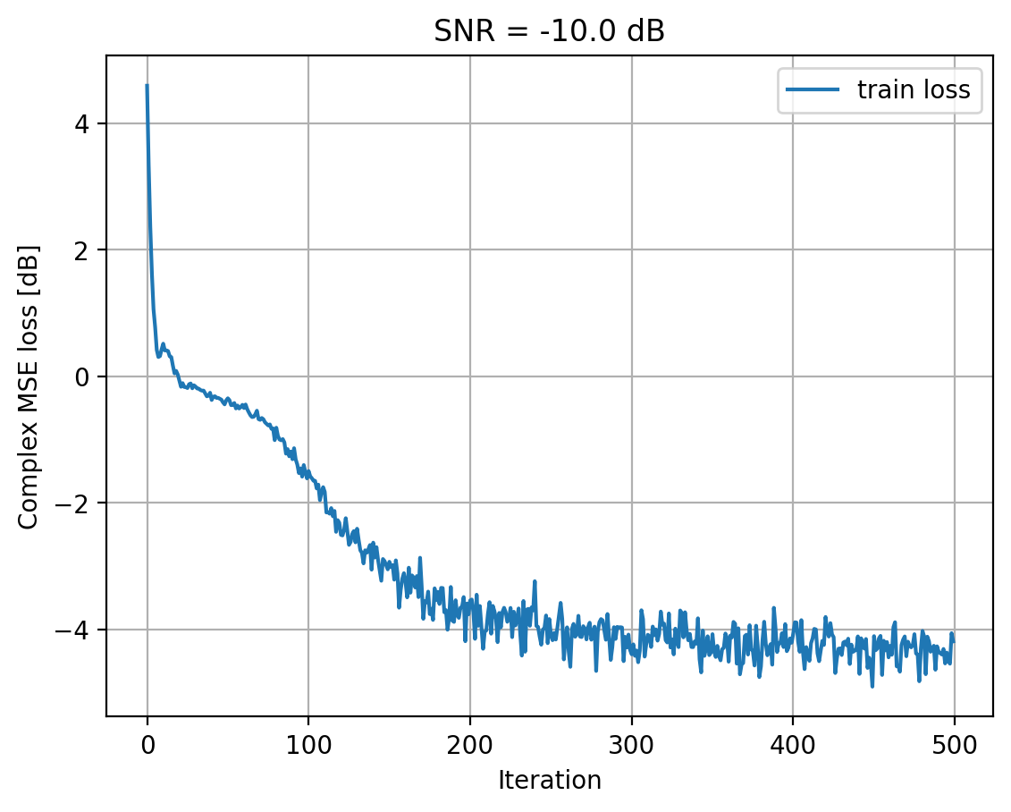
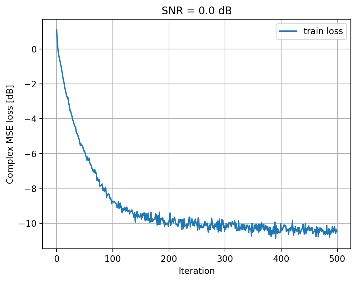
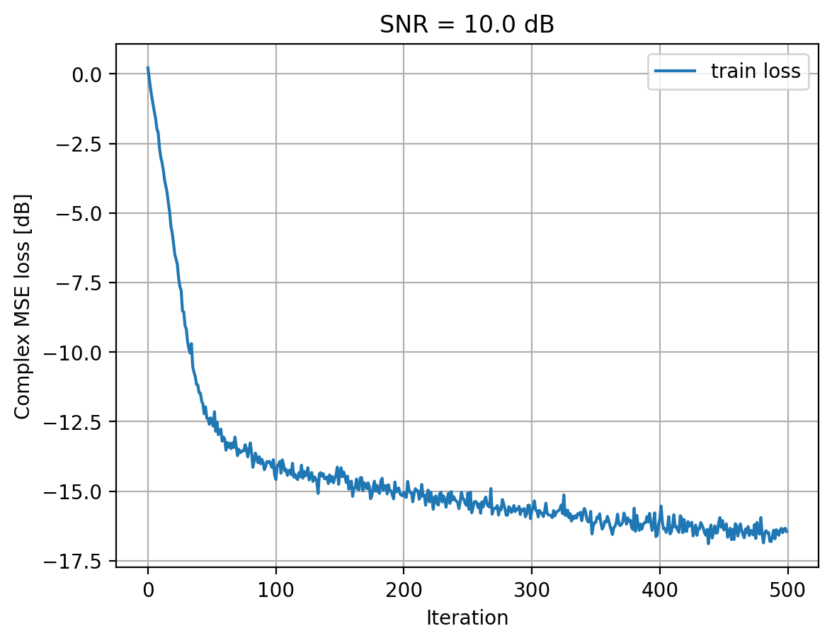
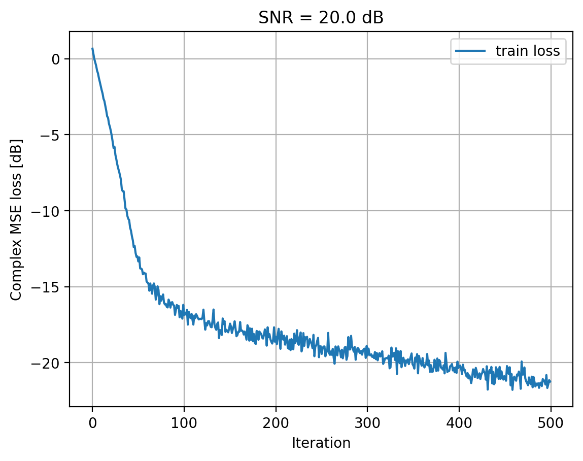
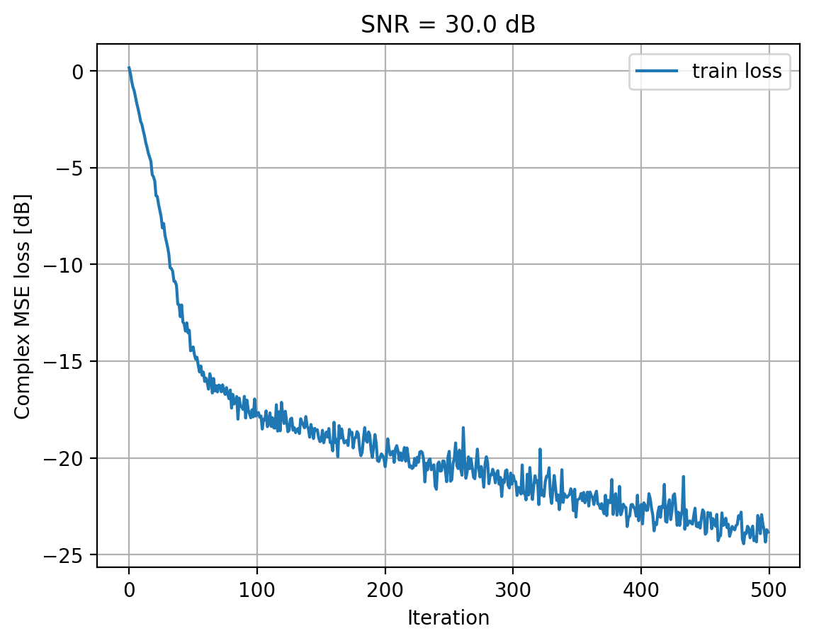
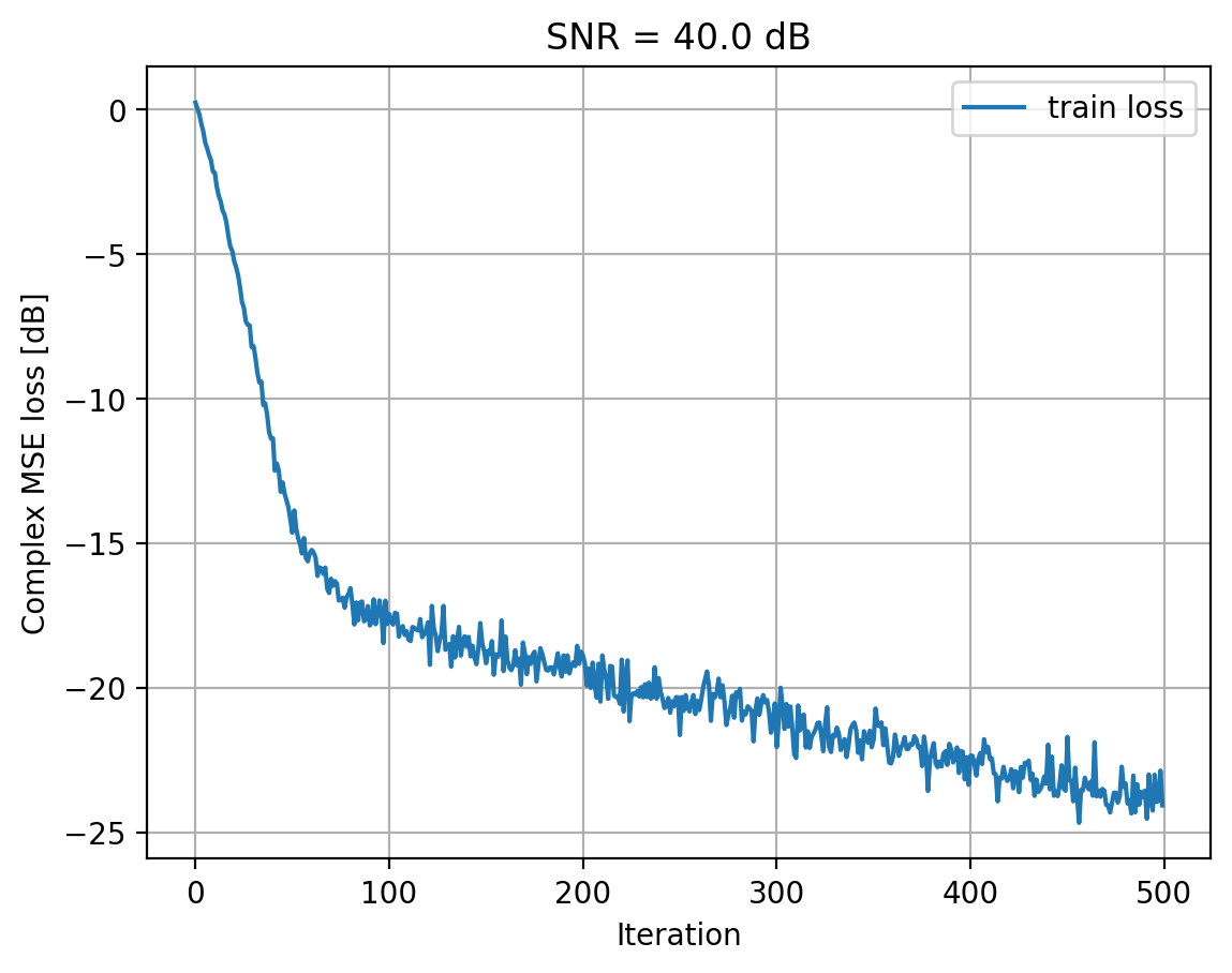
    ut.plot_losses([train_loss], ['train loss'], title=f'SNR ={snr}dB')
        

            

            
XLA can lead to reduced numerical precision. Use with care.
Training model for SNRs: 10 dB
        

            

            
0%|                                                                                                                              | 0/5000 [00:00<?, ?it/s]WARNING: All log messages before absl::InitializeLog() is called are written to STDERR
I0000 00:00:1729133880.135412    9045 device_compiler.h:186] Compiled cluster using XLA!  This line is logged at most once for the lifetime of the process.
Iteration 5000/5000: 100%|████████████████████████████████████████████████████████████████████| 5000/5000 [00:49<00:00, 101.48it/s, Training loss: -20.0 dB]
        

The model trained above is a deep convolutional network, made of RESNET layers, possibly with a fully connected layer at the end in case interpolation is enabled (interp = 2). The diagram for this network is presented below for an example user allocated 48 PRBs:

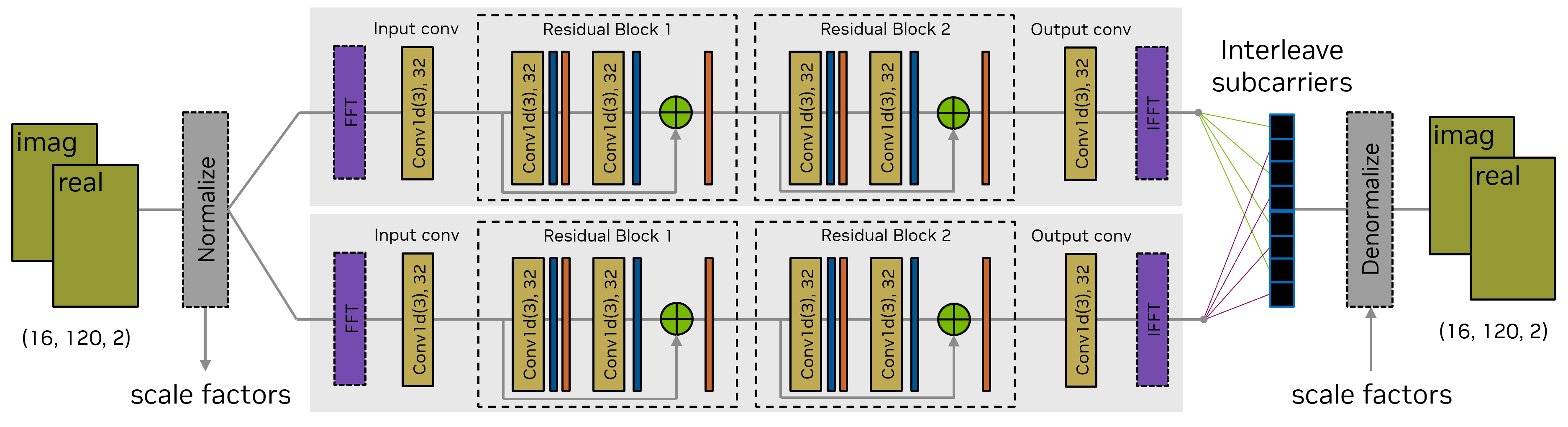
Now we evaluate this network using the LS channel estimates extracted from a PUSCH receiver, as opposed to manually extracted from the channel. The output of the network is compared with MS-MMSE.

            

            
[3]:
        

            

            
train_dir = ut.get_model_training_dir(models_folder, training_ch_model,
                                      num_prbs, n_iter, batch_size)

snr_losses_ls = []             # Least Squares channel estimation losses
snr_losses_ml = []             # Machine learning channel estimation losses
snr_losses_ml2 = []            # Machine learning channel estimation losses (median)

snr_losses_ls_pyaerial = []    # LS from PyAerial
snr_losses_mmse_pyaerial = []  # MMSE from PyAerial
snr_losses_mmse_pyaerial2 = [] # MMSE from PyAerial (median)

# Channel generator for testing
test_ch_gen  = SionnaChannelGenerator(num_prbs, testing_ch_model, batch_size=32)

# Create pyAerial channel estimate generator, using the Sionna Channel Generator
pyaerial_ch_est_gen = PyAerialChannelEstimateGenerator(test_ch_gen)

for snr_idx, snr in enumerate(test_snrs):
    print(f'Testing SNR{snr}dB')

    # Select model trained on the SNR closest to the test SNR
    snr_model_idx = np.argmin(abs(train_snrs - snr))
    snr_model = train_snrs[snr_model_idx]
    print(f'Testing model trained on SNR{snr_model}')

    # Load ML model
    model = ChannelEstimator(num_prbs*12//2, freq_interp_factor=interp).to(dev)
    model.load_state_dict(torch.load(ut.get_snr_model_path(train_dir, snr_model)))

    criterion = ComplexMSELoss()

    model.eval()
    ls_loss, ml_loss, ls_loss_pyaerial, mmse_loss_pyaerial = [], [], [], []
    with torch.no_grad():
        for i in tqdm(range(n_iter_test), desc='Testing LS & MS-MMSE in PyAerial'):
            # Internally generate channels, add noise, receive the DM-RS symbols and estimate the channel
            ls, mmse, gt = pyaerial_ch_est_gen(snr)

            # Evaluate pyAerial classic estimators
            for b in range(len(ls)):
                ls_loss_pyaerial += [ut.complex_mse_loss(ls[b], gt[b][::2])]
                mmse_loss_pyaerial += [ut.complex_mse_loss(mmse[b], gt[b])]

            # Evaluate ML approach
            h, h_ls = torch.tensor(gt).to(dev), torch.tensor(ls).to(dev)
            h_hat = model(h_ls) # h_ls has half the subcarriers of h already
            ls_loss += [criterion(h_ls, h[..., ::2]).item()]
            ml_loss += [criterion(h_hat, h[..., ::(3-interp)]).item()]

    # Compute means and medians of LS, LS+ML and MS-MMSE
    snr_losses_ls += [ut.db(np.mean(ls_loss))]
    snr_losses_ml += [ut.db(np.mean(ml_loss))]
    snr_losses_ml2 += [ut.db(np.median(ml_loss))]

    snr_losses_ls_pyaerial += [ut.db(np.mean(ls_loss_pyaerial))]
    snr_losses_mmse_pyaerial += [ut.db(np.mean(mmse_loss_pyaerial))]
    snr_losses_mmse_pyaerial2 += [ut.db(np.median(mmse_loss_pyaerial))]

    print(f'Avg. ML test loss for{snr}dB SNR is{snr_losses_ml[-1]:.1f}dB')

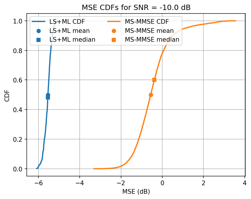
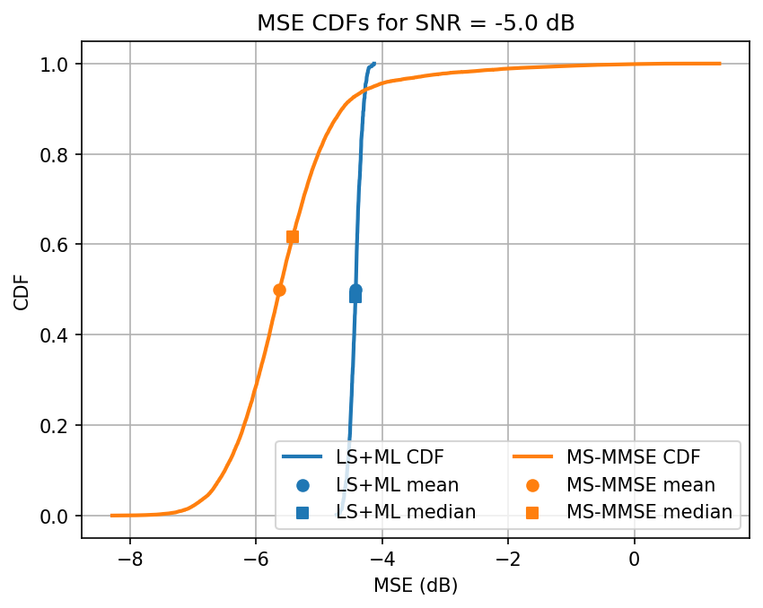
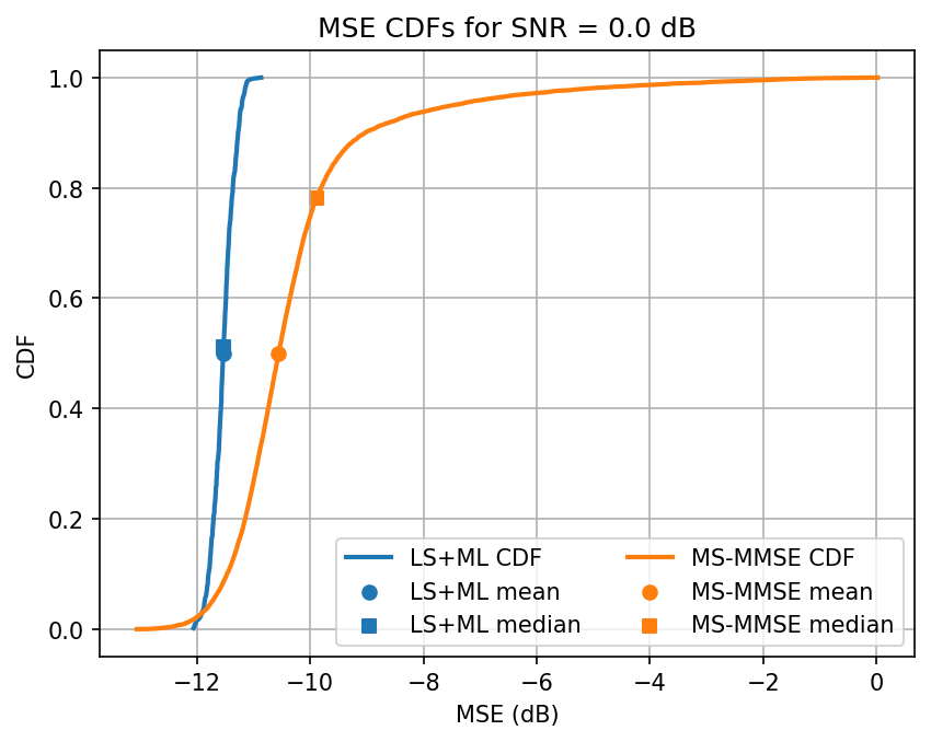
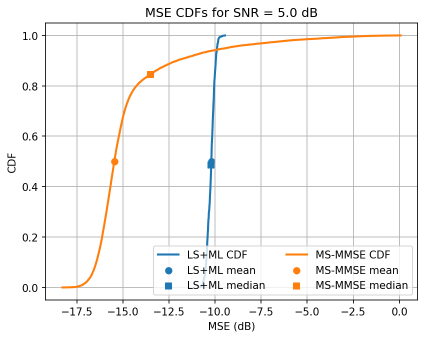
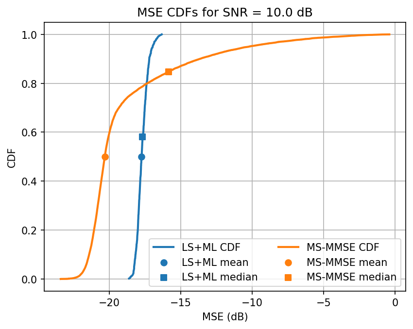
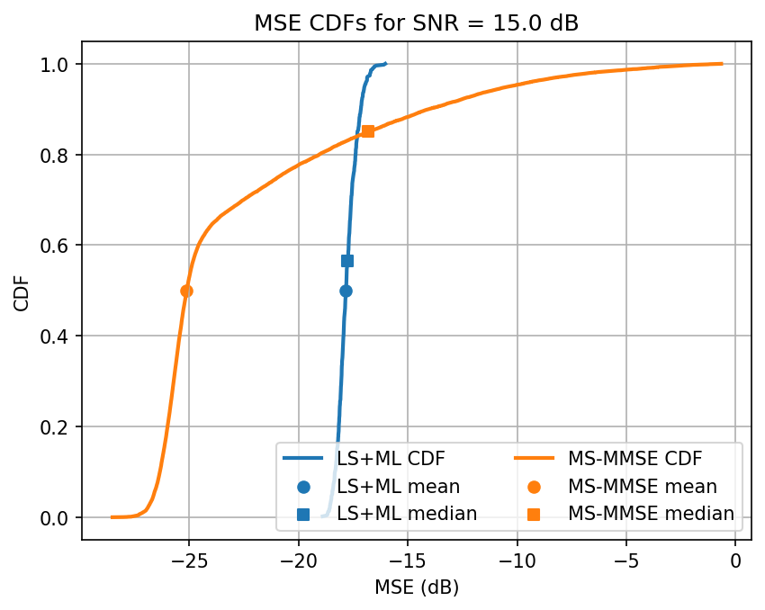
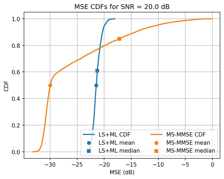
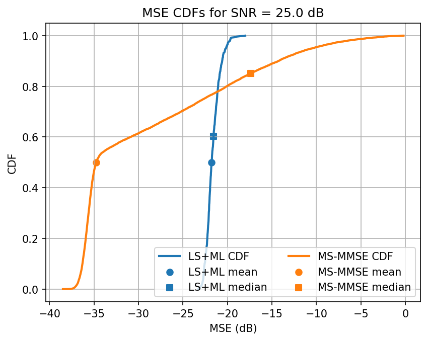
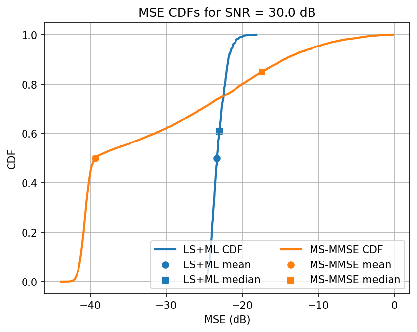
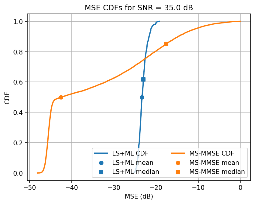
    # Plot CDFs of MSE losses
    ut.plot_annotaded_cdfs([ml_loss, mmse_loss_pyaerial], ['LS+ML', 'MS-MMSE'],
                           title=f'MSE CDFs for SNR ={snr}dB')
        

            

            
XLA can lead to reduced numerical precision. Use with care.
Testing SNR -10.0 dB
Testing model trained on SNR 10
        

            

            
Testing LS & MS-MMSE in PyAerial: 100%|█████████████████████████████████████████████████████████████████████████████████| 1000/1000 [01:11<00:00, 14.01it/s]
        

            

            
Avg. ML test loss for -10.0 dB SNR is 3.2 dB
        

            

            
Testing SNR -5.0 dB
Testing model trained on SNR 10
        

            

            
Testing LS & MS-MMSE in PyAerial: 100%|█████████████████████████████████████████████████████████████████████████████████| 1000/1000 [00:46<00:00, 21.36it/s]
        

            

            
Avg. ML test loss for -5.0 dB SNR is -3.0 dB
        

            

            
Testing SNR 0.0 dB
Testing model trained on SNR 10
        

            

            
Testing LS & MS-MMSE in PyAerial: 100%|█████████████████████████████████████████████████████████████████████████████████| 1000/1000 [00:47<00:00, 21.25it/s]
        

            

            
Avg. ML test loss for 0.0 dB SNR is -10.6 dB
        

            

            
Testing SNR 5.0 dB
Testing model trained on SNR 10
        

            

            
Testing LS & MS-MMSE in PyAerial: 100%|█████████████████████████████████████████████████████████████████████████████████| 1000/1000 [00:46<00:00, 21.39it/s]
        

            

            
Avg. ML test loss for 5.0 dB SNR is -18.4 dB
        

            

            
Testing SNR 10.0 dB
Testing model trained on SNR 10
        

            

            
Testing LS & MS-MMSE in PyAerial: 100%|█████████████████████████████████████████████████████████████████████████████████| 1000/1000 [00:46<00:00, 21.33it/s]
        

            

            
Avg. ML test loss for 10.0 dB SNR is -22.1 dB
        

            

            
Testing SNR 15.0 dB
Testing model trained on SNR 10
        

            

            
Testing LS & MS-MMSE in PyAerial: 100%|█████████████████████████████████████████████████████████████████████████████████| 1000/1000 [00:46<00:00, 21.39it/s]
        

            

            
Avg. ML test loss for 15.0 dB SNR is -23.0 dB
        

            

            
Testing SNR 20.0 dB
Testing model trained on SNR 10
        

            

            
Testing LS & MS-MMSE in PyAerial: 100%|█████████████████████████████████████████████████████████████████████████████████| 1000/1000 [00:46<00:00, 21.36it/s]
        

            

            
Avg. ML test loss for 20.0 dB SNR is -23.3 dB
        

            

            
Testing SNR 25.0 dB
Testing model trained on SNR 10
        

            

            
Testing LS & MS-MMSE in PyAerial: 100%|█████████████████████████████████████████████████████████████████████████████████| 1000/1000 [00:46<00:00, 21.38it/s]
        

            

            
Avg. ML test loss for 25.0 dB SNR is -23.3 dB
        

            

            
Testing SNR 30.0 dB
Testing model trained on SNR 10
        

            

            
Testing LS & MS-MMSE in PyAerial: 100%|█████████████████████████████████████████████████████████████████████████████████| 1000/1000 [00:46<00:00, 21.36it/s]
        

            

            
Avg. ML test loss for 30.0 dB SNR is -23.4 dB
        

            

            
Testing SNR 35.0 dB
Testing model trained on SNR 10
        

            

            
Testing LS & MS-MMSE in PyAerial: 100%|█████████████████████████████████████████████████████████████████████████████████| 1000/1000 [00:46<00:00, 21.39it/s]
        

            

            
Avg. ML test loss for 35.0 dB SNR is -23.4 dB
        

            

            
Testing SNR 40.0 dB
Testing model trained on SNR 10
        

            

            
Testing LS & MS-MMSE in PyAerial: 100%|█████████████████████████████████████████████████████████████████████████████████| 1000/1000 [00:46<00:00, 21.36it/s]
        

            

            
Avg. ML test loss for 40.0 dB SNR is -23.3 dB
        

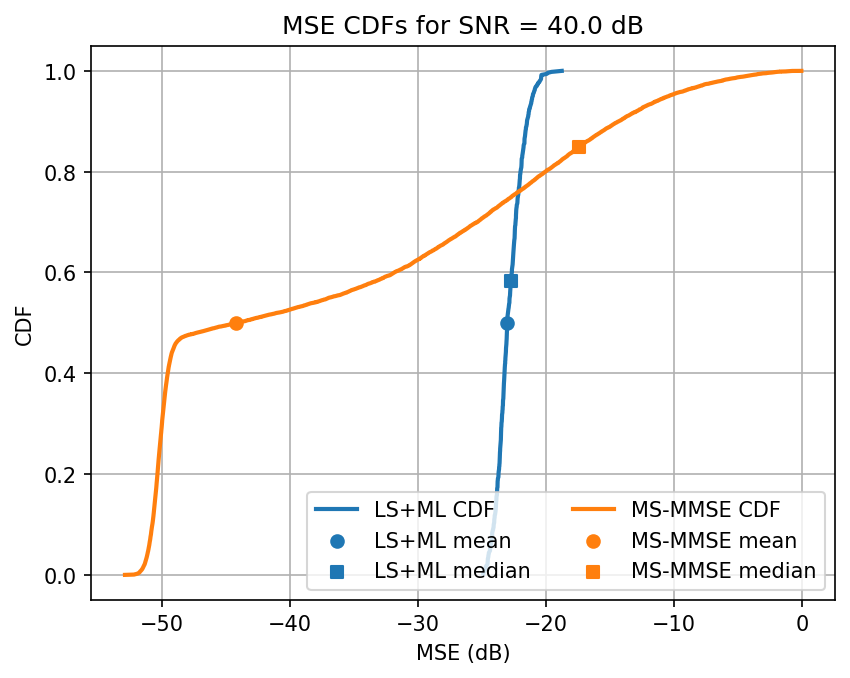
Observation: When we fine tune our training, we see the ML model outperforming the MS-MMSE approach for most SNRs. The performance decays slightly when interpolation is necessary. Additionally, the ML seems more reliable for a wider class of channels. The variance of estimates is lower for ML, on average, it’s performance saturates for high SNRs, even if the median continues to decay.

Requirement: test_snrs must have more than one element. Read below why we would want to do this.

Model switching depending on SNR: One of the challenges in channel estimation is having it work across SNRs. Lower SNRs have higher channel estimation mean squared error (MSE), which influences more heavily the loss of these samples in machine learning models, thus leading the model learn only low-SNR channels. One way to avoid this problem is to do a model-switching approach. In model-switching, each model is trained for a single SNR and use the model that has the closest SNR to the SNR of the user.

Note that this approach requires a sufficiently good estimate of the SNR so the correct model is chosen. Usually, acquiring such an estimate is not difficult - for example, using the MMSE channel estimate should have more resolution than needed. As such, here we assume the SNR of the user is known and the closest model is selected.

If we set train_snrs = [-10, 0, 10, 20, 30, 40] and test_snrs = [-10, -5, 0, 5, 10, 15, ..., 40], then we will see that the model trained for an SNR of -10 dB is also used to estimate channels at -5 dB, and the model trained for 0 dB is also used at 5 dB, etc. This leads to a higher MSE in SNRs divisible by 5 but not 10.

            

            
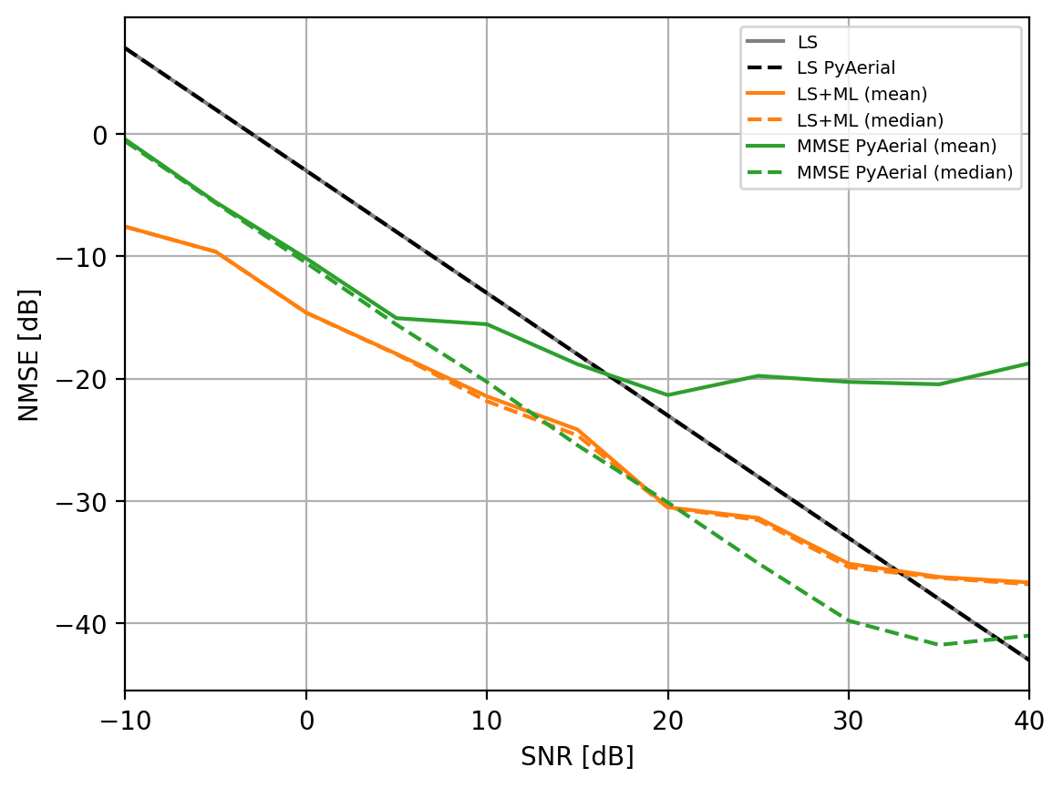
[4]:
        

            

            
plt.figure(dpi=200)

plt.plot(test_snrs, snr_losses_ls,              '-', label='LS',                     color ='k', alpha=.7)
plt.plot(test_snrs, snr_losses_ls_pyaerial,    '--', label='LS PyAerial',            color ='k')
plt.plot(test_snrs, snr_losses_ml,              '-', label='LS+ML (mean)',           color ='tab:orange')
plt.plot(test_snrs, snr_losses_ml2,            '--', label='LS+ML (median)',         color ='tab:orange')
plt.plot(test_snrs, snr_losses_mmse_pyaerial,   '-', label='MMSE PyAerial (mean)',   color ='tab:green')
plt.plot(test_snrs, snr_losses_mmse_pyaerial2, '--', label='MMSE PyAerial (median)', color ='tab:green')

plt.xlabel('SNR [dB]')
plt.ylabel('NMSE [dB]')
plt.xlim((min(test_snrs), max(test_snrs)))
plt.legend(fontsize=7)
plt.grid()
plt.show()
        

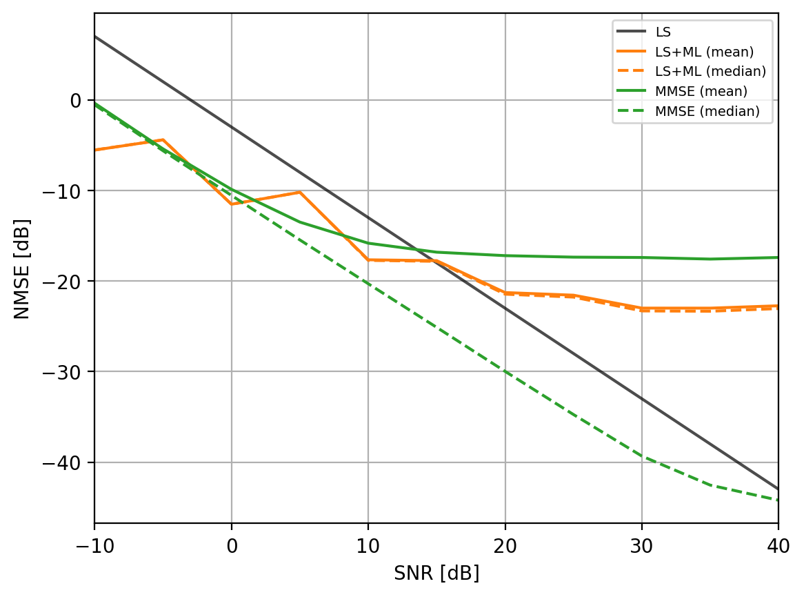
Below is an example of this plot for the case interp = 2 and 48 PRBs.

Some noteworthy gains compared to MS-MMSE:

• 5-8 dB gain for SNRs \(\in [-10, 0]\) dB

• 3-5 dB gain for SNRs \(\in [ 0, 10]\) dB

• 0-3 dB gain for SNRs \(\in [10, 20]\) dB

• after 10 dB, the ML model is comparatively more reliable, with a more predictable CDF and better average performance

Note that this approach is expected to work better for higher PRB allocations. Likely due to being to extract more information from the channel. The model also has better performance when interp = 1 since interpolation is not necessary, which makes the network harder to train by the addition of the fully connected at the end.

Considerations for Real Deployments

For such approach to work in real deployments, it requires two additional steps we choose to omit here for simplicity: - SNR estimation: required to estimate the optimized model to perform channel estimation. Here, we consider the SNR is known. - PRB parallelization: during inference, the PRB parallelizer would split the LS estimates (e.g. 78 PRBs) into chunks that could be processed in parallel by the trained models of different sizes, and then put back together. As an example, if we trained models for {1, 4, 16} PRBs, the 78 PRB estimate would results in 4 batches for the 16 PRB model, 3 batches for the 4 PRB and 2 batches for the 1 PRB (4 * 16 + 3 * 4 + 2*1 = 64 + 12 + 2 = 78)

Assessing System-level Performance in the Aerial Omniverse Digital Twin

This notebook can be used to generate models compatible with the machine learning example of PUSCH channel estimation in the AODT. As long as the models_folder variable is kept constant across runs, a single folder will be populated with the correct structure for multiple SNRs and PRBs. As mentioned in the AODT user guide, this folder will then need to be moved to a directory accessible by the AODT backend, and the config_est.ini file populated with the absolute path to the folder.

Benefits of using PyAerial as a bridge to AODT

• AODT uses a high-performance EM solver for computing raytracing propagation simulations. Raytracing is necessary for studying ML approaches in site-specific settings, offering insight and explainability to edge-cases previously unavailable in stochastic simulations.

• AODT RAN simulations use the same software running on the same hardware deployed in the real world. This unprecedented combination creates an accurate system representation, giving researchers the possibility to design new features (AI/ML powered or not) and assess their network-wide end-to-end impact.

• PyAerial currently provides a Python interface only to cuPHY, the PHY layer of Aerial. As such, comparions beyond the PHY are not possible in PyAerial, and the last link-level quantity that can be computed is block error rates. The AODT, on the other hand, integrates both Aerial’s cuPHY and cuMAC, allowing researchers to measure how channel estimation impacts higher layers.

For more information about how to run this ML channel estimation in AODT, see the AODT user guide.