Advanced Performance Measurement Techniques

Before starting any optimization effort with TensorRT, it is essential to determine what should be measured. Without measurements, it is impossible to make reliable progress or measure whether success has been achieved.

Latency: A performance measurement for network inference is how much time elapses from an input presented to the network until an output is available. This is the latency of the network for a single inference. Lower latencies are better. In some applications, low-latency is a critical safety requirement. In other applications, latency is directly visible to users as a quality-of-service issue. For bulk processing, latency cannot be important.

Throughput: Another performance measurement is how many inferences can be completed in a fixed time. This is the throughput of the network. Higher throughput is better. Higher throughputs indicate a more efficient utilization of fixed compute resources. For bulk processing, the total time taken will be determined by the network’s throughput.

Another way of looking at latency and throughput is to fix the maximum latency and measure throughput at that latency. A quality-of-service measurement like this can be a reasonable compromise between the user experience and system efficiency.

Before measuring latency and throughput, you must choose the exact points to start and stop timing. Different points make sense depending on the network and application.

In many applications, there is a processing pipeline, and the latency and throughput of the entire pipeline can measure the overall system performance. Because the pre-and post-processing steps depend so strongly on the particular application, this section considers the latency and throughput of the network inference only.

Wall-Clock Timing

The wall clock time (the elapsed time between the start of a computation and its end) can be useful for measuring the application’s overall throughput and latency and placing inference times in context within a larger system. To measure wall clock time, we can use std::chrono::steady_clock provided by the C++11 <chrono> standard library.

The following example code snippet shows measuring network inference host time:

C++

#include <chrono>

auto startTime = std::chrono::steady_clock::now();
context->enqueueV3(stream);
cudaStreamSynchronize(stream);
auto endTime = std::chrono::steady_clock::now();
float totalTime = std::chrono::duration<float, std::milli>
    (endTime - startTime).count();

Python

import time
from cuda import cudart
err, stream = cudart.cudaStreamCreate()
start_time = time.time()
context.execute_async_v3(stream)
cudart.cudaStreamSynchronize(stream)
total_time = time.time() - start_time

If there is only one inference happening on the device at one time, then this can be a simple way of profiling the time-various operations take. Inference is typically asynchronous, so ensure you add an explicit CUDA stream or device synchronization to wait for results to become available.

CUDA Events

One problem with timing on the host exclusively is that it requires host/device synchronization. Optimized applications can have many inferences running parallel on the device with overlapping data movement. In addition, the synchronization adds some noise to timing measurements.

To help with these issues, CUDA provides an Event API. This API allows you to place events into CUDA streams that the GPU will time-stamp as they are encountered. Differences in timestamps can then tell you how long different operations took.

The following example code snippet shows computing the time between two CUDA events:

C++

cudaEvent_t start, end;
cudaEventCreate(&start);
cudaEventCreate(&end);

cudaEventRecord(start, stream);
context->enqueueV3(stream);
cudaEventRecord(end, stream);

cudaEventSynchronize(end);
float totalTime;
cudaEventElapsedTime(&totalTime, start, end);

Python

from cuda import cudart
err, stream = cudart.cudaStreamCreate()
err, start = cudart.cudaEventCreate()
err, end = cudart.cudaEventCreate()
cudart.cudaEventRecord(start, stream)
context.execute_async_v3(stream)
cudart.cudaEventRecord(end, stream)
cudart.cudaEventSynchronize(end)
err, total_time = cudart.cudaEventElapsedTime(start, end)

Built-In TensorRT Profiling

Digging deeper into inference performance requires more fine-grained timing measurements within the optimized network.

TensorRT has a Profiler (C++, Python) interface, which you can implement to have TensorRT pass profiling information to your application. When called, the network will run in a profiling mode. After finishing the inference, the profiler object of your class is called to report the timing for each layer in the network. These timings can be used to locate bottlenecks, compare different versions of a serialized engine, and debug performance issues.

The profiling information can be collected from a regular inference enqueueV3() launch or a CUDA graph launch. Refer to IExecutionContext::setProfiler() and IExecutionContext::reportToProfiler() (C++, Python) for more information.

Layers inside a loop are compiled into a single monolithic layer; therefore, separate timings for those layers are unavailable. Also, some subgraphs (especially with Transformer-like networks) are handled by a next-generation graph optimizer that has not yet been integrated with the Profiler APIs. For those networks, use the CUDA Profiling Tools to profile per-layer performance.

An example showing how to use the IProfiler interface is provided in the common sample code (common.h).

Given an input network or plan file, you can use trtexec to profile a network with TensorRT. For more information, refer to the trtexec section.

ONNX Profiling Tools

Nsight Deep Learning Designer is an integrated design environment for ONNX models. It is built on top of TensorRT. Its built-in profiler runs inference for an ONNX model through TensorRT and collects profiling data based on GPU performance metrics. The profiler report generated by Nsight Deep Learning Designer provides a comprehensive view of an ONNX model’s inference performance at the TensorRT layer level. Its GUI also helps developers correlate the performance of individual TensorRT layers with their originating ONNX operators.

Nsight Deep Learning Designer profiling typically begins with the GUI. Open the Nsight Deep Learning Designer application and click Start Activity from the Welcome screen. Select the target platform type from the list, and you can also define a remote connection to profile on a Linux or L4T target from a remote machine. Select Profile TensorRT Model as the activity type.

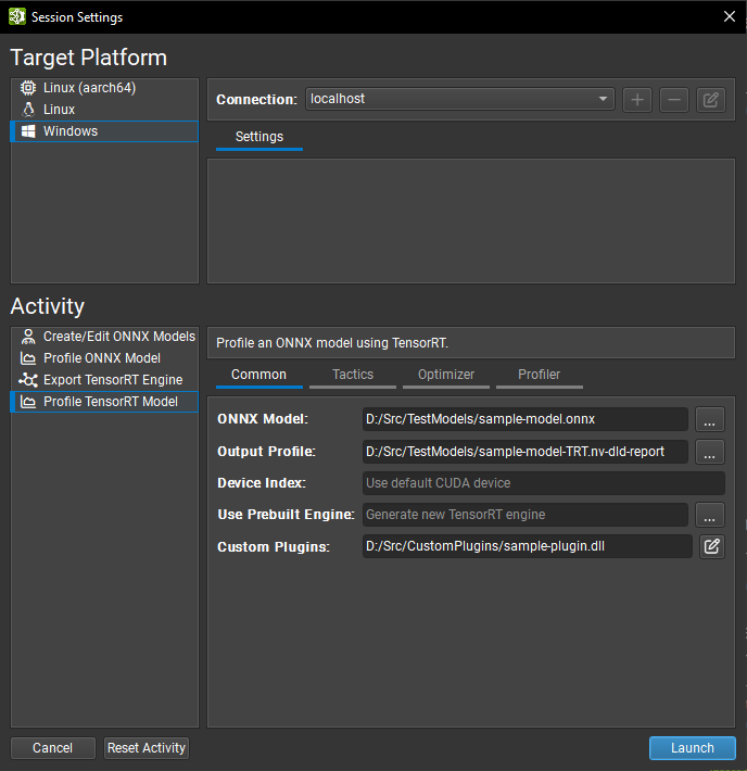
Profiler activity settings typically have analogs in trtexec and are split across four tabs in the GUI. Refer to the Nsight Deep Learning Designer documentation for details of each setting. The most frequently used settings are listed here:

• Common: The ONNX model to profile, its corresponding TensorRT engine if one has already been built, and the location to save the profiler report.

• Tactics: Typing mode (default typing, type constraints (Layer-Level Control of Permission), or strong typing (Strongly Typed Networks)) and on/off toggles for FP16, BF16, TF32, INT8, and FP8 precisions in weakly typed networks (Network-Level Control of Precision).

• Optimizer: Refittable weights (Refitting an Engine), INT8 quantization cache path (Post-Training Quantization Using Calibration).

• Profiler: Locking GPU clocks to base values (GPU Clock Locking and Floating Clock) and GPU counter sampling rate.

Networks using dynamic shapes (Working with Dynamic Shapes) should specify an optimization profile before profiling. This can be done by editing the ONNX network within Nsight Deep Learning Designer, profiling from the command line, or (for compatible networks) setting the Inferred Batch option in the Optimizer tab. When a batch size is provided, input shapes with a single leading wildcard will be automatically populated with the batch size. This feature works with input shapes of arbitrary rank.

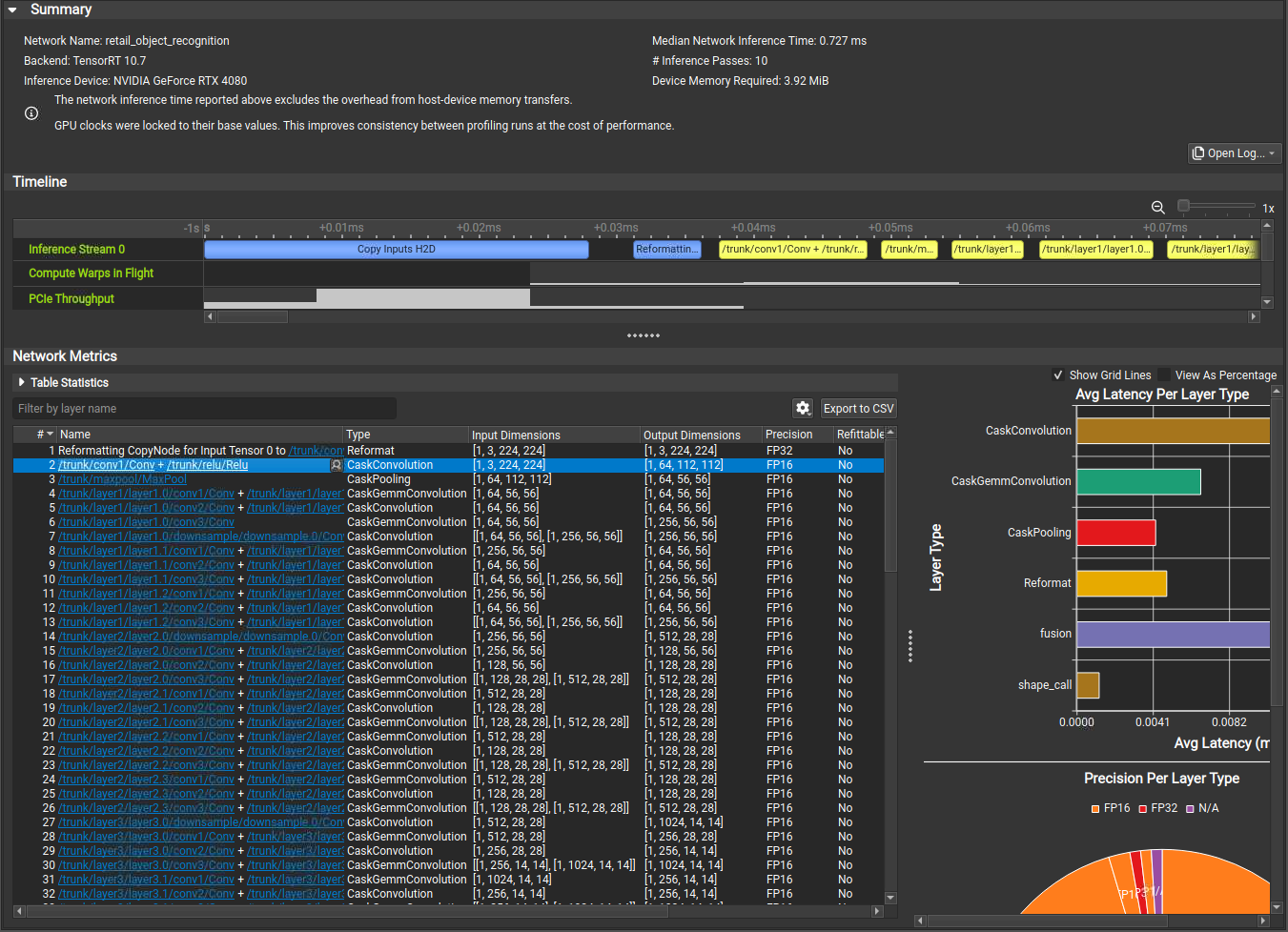
To start the Nsight Deep Learning Designer profiler, click the Launch button. The tool will automatically deploy TensorRT and CUDA runtime libraries to the target as needed and then generate a profiling report:

Nsight Deep Learning Designer includes a command-line profiler; refer to the tool documentation for usage instructions.

Understanding Nsight Deep Learning Designer Timeline View

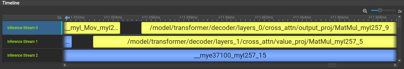
In the Nsight Deep Learning Designer Timeline View, each network inference stream is shown as a row of the timeline alongside collected GPU metrics such as SM activity and PCIe throughput. Each layer executed on an inference stream is depicted as a range on the corresponding timeline view. Overhead sources such as tensor memory copies or reformats are highlighted in blue.

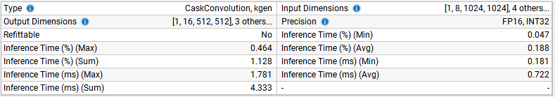
Understanding Nsight Deep Learning Designer Layer Table

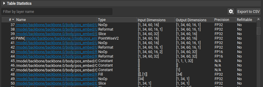
The Network Metrics table view shows all TensorRT layers executed by the network, their type, dimensions, precision, and inference time. Layer inference times are provided in the table as both raw time measurements and percentages of the inference pass. You can filter the table by name. Hyperlinks in the table indicate where a layer name references nodes in the original ONNX source model. Click the hyperlink or use the drop-down menu in a selected layer’s Name column to open the original ONNX model and highlight the layer in its context.

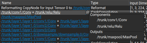
Selecting a range of layers in the table aggregates their statistics into a higher-level summary. Each table column is represented in the summary area with the most common values observed within the selection, sorted by frequency. Hover the mouse cursor over an information icon to view the full list of values and associated frequencies. Inference time columns are shown as minimum, maximum, mean, and total, using absolute times, and inference pass percentages as units. Total times in this context can be used to quickly sum the inference time for layers within a single execution stream. Layers in the selection do not need to be contiguous.

Understanding Nsight Deep Learning Designer Network Graphs

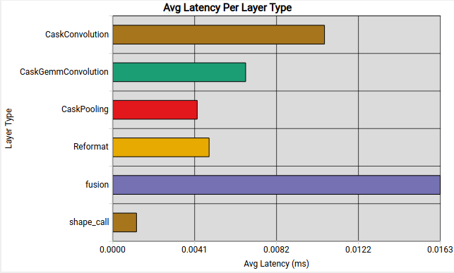
Nsight Deep Learning Designer shows the average inference latency for each type of layer in the TensorRT engine. This can highlight areas where the network spends significant time on non-critical computations.

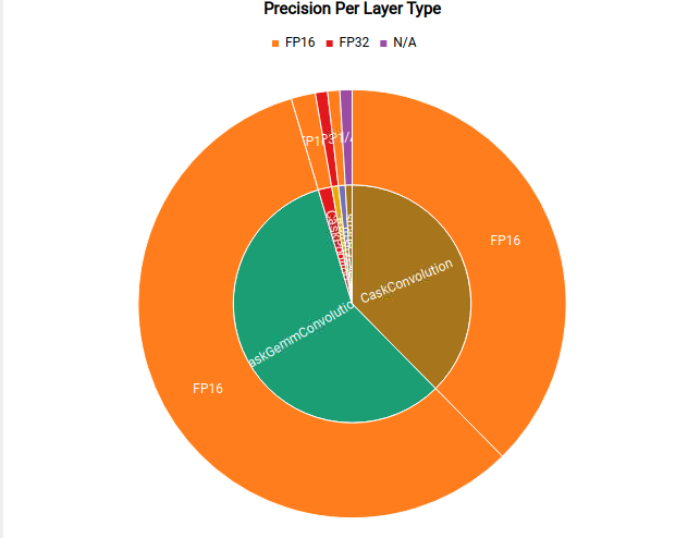
Nsight Deep Learning Designer also shows the precisions used for each type of layer in the TensorRT engine. This can highlight potential opportunities for network quantization and visualize the effect of setting TensorRT’s tactic precision flags.

CUDA Profiling Tools

The recommended CUDA profiler is NVIDIA Nsight Systems. Some CUDA developers can be more familiar with nvprof and nvvp. However, these are being deprecated. These profilers can be used on any CUDA program to report timing information about the kernels launched during execution, data movement between host and device, and CUDA API calls used.

Nsight Systems can be configured to report timing information for only a portion of the program’s execution or to report traditional CPU sampling profile information and GPU information.

The basic usage of Nsight Systems is first to run the command nsys profile -o <OUTPUT> <INFERENCE_COMMAND>, then open the generated <OUTPUT>.nsys-rep file in the Nsight Systems GUI to visualize the captured profiling results.

Profile Only the Inference Phase

When profiling a TensorRT application, you should enable profiling only after the engine has been built. During the build phase, all possible tactics are tried and timed. Profiling this portion of the execution will not show any meaningful performance measurements and will include all possible kernels, not the ones selected for inference. One way to limit the scope of profiling is to:

• First phase: Structure the application to build and then serialize the engines in one phase.

• Second phase: Load the serialized engines, run inference in a second phase, and profile this second phase only.

Suppose the application cannot serialize the engines or must run through the two phases consecutively. In that case, you can also add cudaProfilerStart() and cudaProfilerStop() CUDA APIs around the second phase and add the -c cudaProfilerApi flag to the Nsight Systems command to profile only the part between cudaProfilerStart() and cudaProfilerStop().

Understand Nsight Systems Timeline View

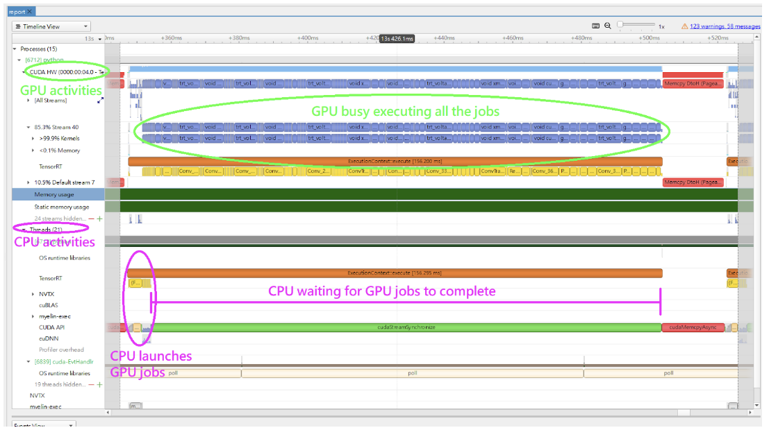
In the Nsight Systems Timeline View, the GPU activities are shown in the rows under CUDA HW, and the CPU activities are shown in the rows under Threads. By default, the rows under CUDA HW are collapsed. Therefore, you must click on it to expand the rows.

In a typical inference workflow, the application calls the context->enqueueV3() or context->executeV3() APIs to enqueue the jobs and then synchronize on the stream to wait until the GPU completes the jobs. If you only look at the CPU activities, it can appear that the system is idle for an extended period in the cudaStreamSychronize() call. The GPU can be busy executing the enqueued jobs while the CPU waits. The following figure shows an example timeline of the inference of a query.

The trtexec tool uses a slightly more complicated approach to enqueue the jobs. It enqueues the next query while the GPU still executes the jobs from the previous query. For more information, refer to the trtexec section.

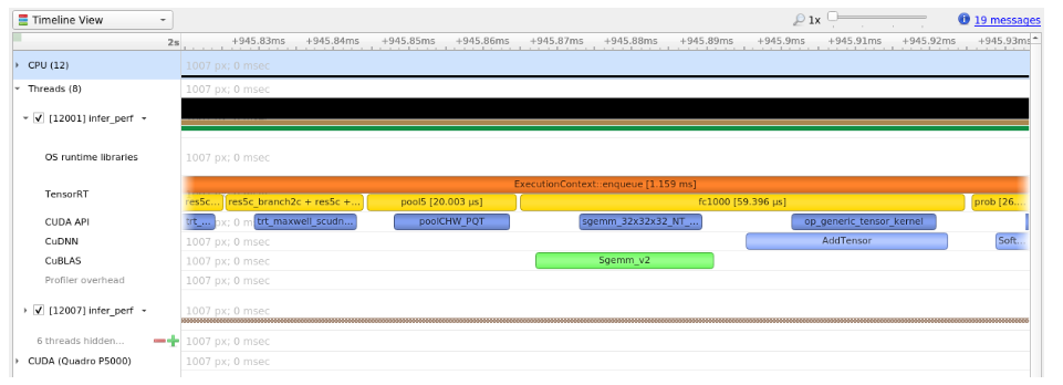
The following image shows a typical view of the normal inference workloads in the Nsight Systems timeline view, showing CPU and GPU activities on different rows.

Use the NVTX Tracing in Nsight Systems

Tracing enables the NVIDIA Tools Extension SDK (NVTX), a C-based API for marking events and ranges in your applications. It allows Nsight Compute and Nsight Systems to collect data generated by TensorRT applications.

Decoding the kernel names back to layers in the original network can be complicated. Because of this, TensorRT uses NVTX to mark a range for each layer, allowing the CUDA profilers to correlate each layer with the kernels called to implement it. In TensorRT, NVTX helps to correlate the runtime engine layer execution with CUDA kernel calls. Nsight Systems supports collecting and visualizing these events and ranges on the timeline. Nsight Compute also supports collecting and displaying the state of all active NVTX domains and ranges in a given thread when the application is suspended.

In TensorRT, each layer can launch one or more kernels to perform its operations. The exact kernels launched depend on the optimized network and the hardware present. Depending on the builder’s choices, multiple additional operations that reorder data can be interspersed with layer computations; these reformat operations can be implemented as device-to-device memory copies or custom kernels.

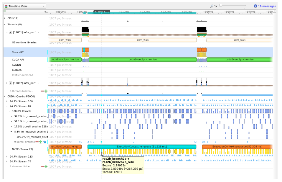
For example, the following screenshots are from Nsight Systems.

The kernels run on the GPU; in other words, the following image shows the correlation between the layer execution and kernel launch on the CPU side and their execution on the GPU side.

Control the Level of Details in NVTX Tracing

By default, TensorRT only shows layer names in the NVTX markers. At the same time, users can control the level of details by setting the ProfilingVerbosity in the IBuilderConfig when the engine is built. For example, to disable NVTX tracing, set the ProfilingVerbosity to kNONE:

C++

builderConfig->setProfilingVerbosity(ProfilingVerbosity::kNONE);

Python

builder_config.profilling_verbosity = trt.ProfilingVerbosity.NONE

On the other hand, you can choose to allow TensorRT to print more detailed layer information in the NVTX markers, including input and output dimensions, operations, parameters, tactic numbers, and so on, by setting the ProfilingVerbosity to kDETAILED:

C++

builderConfig->setProfilingVerbosity(ProfilingVerbosity::kDETAILED);

Python

builder_config.profilling_verbosity = trt.ProfilingVerbosity.DETAILED

Note

Enabling detailed NVTX markers increases the latency of enqueueV3() calls and could result in a performance drop if the performance depends on the latency of enqueueV3() calls.

Run Nsight Systems with trtexec

Below is an example of the commands to gather Nsight Systems profiles using the trtexec tool:

trtexec --onnx=foo.onnx --profilingVerbosity=detailed --saveEngine=foo.plan
nsys profile -o foo_profile --capture-range cudaProfilerApi trtexec --profilingVerbosity=detailed --loadEngine=foo.plan --warmUp=0 --duration=0 --iterations=50

The first command builds and serializes the engine to foo.plan, and the second command runs the inference using foo.plan and generates a foo_profile.nsys-rep file that can then be opened in the Nsight Systems user interface for visualization.

The --profilingVerbosity=detailed flag allows TensorRT to show more detailed layer information in the NVTX marking, and the --warmUp=0, --duration=0, and --iterations=50 flags allow you to control how many inference iterations to run. By default, trtexec runs inference for three seconds, which can result in a large output of the nsys-rep file.

If the CUDA graph is enabled, add --cuda-graph-trace=node flag to the nsys command to view the per-kernel runtime information:

nsys profile -o foo_profile --capture-range cudaProfilerApi --cuda-graph-trace=node trtexec --profilingVerbosity=detailed --loadEngine=foo.plan --warmUp=0 --duration=0 --iterations=50 --useCudaGraph

Optional: Enable GPU Metrics Sampling in Nsight Systems

On discrete GPU systems, add the --gpu-metrics-device all flag to the nsys command to sample GPU metrics, including GPU clock frequencies, DRAM bandwidth, Tensor Core utilization. If the flag is added, these GPU metrics appear in the Nsight Systems web interface.

Profiling for DLA

To profile DLA, add the --accelerator-trace nvmedia flag when using the NVIDIA Nsight Systems CLI or enable Collect other accelerators trace when using the user interface. For example, the following command can be used with the NVIDIA Nsight Systems CLI:

nsys profile -t cuda,nvtx,nvmedia,osrt --accelerator-trace=nvmedia  --show-output=true trtexec --loadEngine=alexnet_int8.plan --warmUp=0 --duration=0 --iterations=20

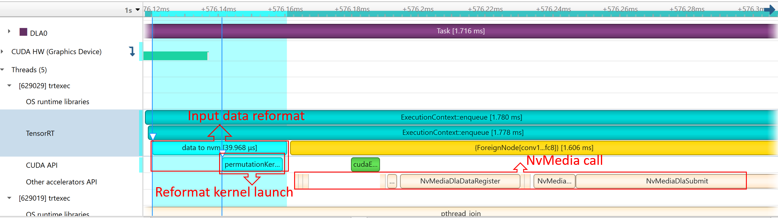
Here is an example report:

• NvMediaDLASubmit submits a DLA task for each DLA subgraph. The task’s runtime can be found in the DLA timeline under Other accelerators trace.

• Because GPU fallback was allowed, TensorRT automatically added some CUDA kernels, like permutationKernelPLC3 and copyPackedKernel, which are used for data reformatting.

• EGLStream APIs were executed because TensorRT uses EGLStream for data transfer between GPU memory and DLA.

To maximize GPU utilization, trtexec enqueues the queries one batch beforehand.

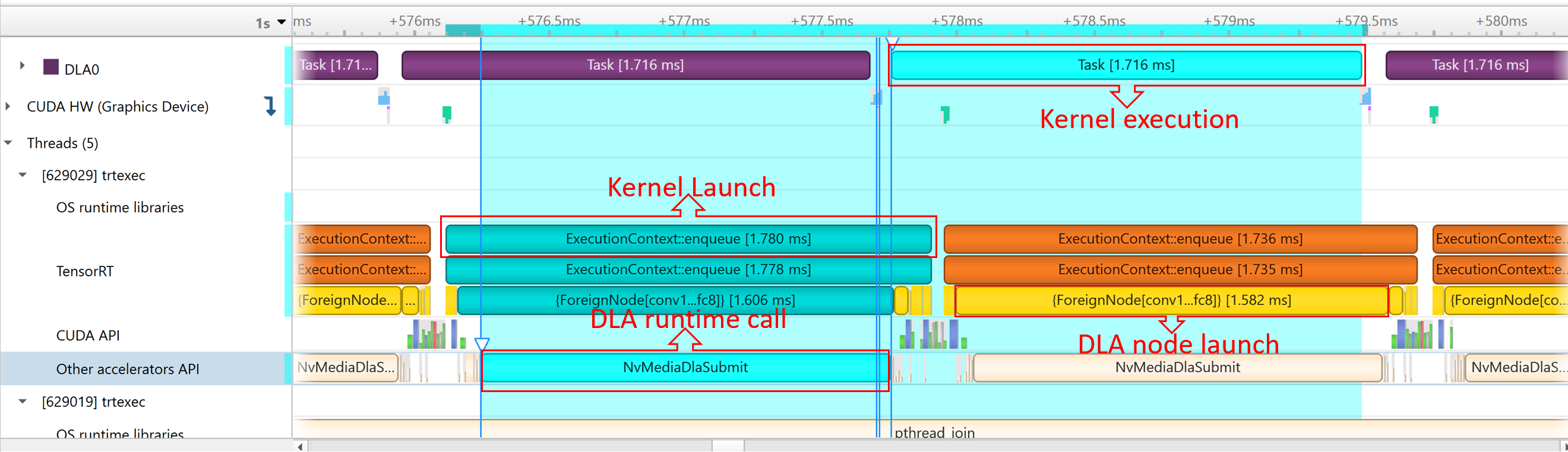
The runtime of the DLA task can be found under Other Accelerator API. Some CUDA kernels and EGLStream API are called for interaction between GPU and DLA.

Tracking Memory

Tracking memory usage can be as important as execution performance. Usually, the device’s memory is more constrained than the host’s. To keep track of device memory, the recommended mechanism is to create a simple custom GPU allocator that internally keeps some statistics and then uses the regular CUDA memory allocation functions cudaMalloc and cudaFree.

A custom GPU allocator can be set for the builder IBuilder for network optimizations and IRuntime when deserializing engines using the IGpuAllocator APIs. One idea for the custom allocator is to keep track of the current amount of memory allocated and push an allocation event with a timestamp and other information onto a global list of allocation events. Looking through the list of allocation events allows profiling memory usage over time.

On mobile platforms, GPU memory and CPU memory share the system memory. On devices with very limited memory size, like Nano, system memory might run out with large networks; even the required GPU memory is smaller than system memory. In this case, increasing the system swap size could solve some problems. An example script is:

echo "######alloc swap######"
if [ ! -e /swapfile ];then
    sudo fallocate -l 4G /swapfile
    sudo chmod 600 /swapfile
    sudo mkswap /swapfile
    sudo /bin/sh -c 'echo  "/swapfile \t none \t swap \t defaults \t 0 \t 0" >> /etc/fstab'
    sudo swapon -a
fi