Scalar Transport: 2D Advection Diffusion#
Introduction#
In this tutorial, you will use an advection-diffusion transport equation for temperature along with the Continuity and Navier-Stokes equation to model the heat transfer in a 2D flow. In this tutorial you will learn:
How to implement advection-diffusion for a scalar quantity.
How to create custom profiles for boundary conditions and to set up gradient boundary conditions.
How to use additional constraints like
IntegralBoundaryConstraintto speed up convergence.
Note
This tutorial assumes that you have completed tutorial Introductory Example and have familiarized yourself with the basics of the PhysicsNeMo Sym APIs.
Problem Description#
In this tutorial, you will solve the heat transfer from a 3-fin heat sink. The problem describes a hypothetical scenario wherein a 2D slice of the heat sink is simulated as shown in the figure. The heat sinks are maintained at a constant temperature of 350 \(K\) and the inlet is at 293.498 \(K\). The channel walls are treated as adiabatic. The inlet is assumed to be a parabolic velocity profile with 1.5 \(m/s\) as the peak velocity. The kinematic viscosity \(\nu\) is set to 0.01 \(m^2/s\) and the Prandtl number is 5. Although the flow is laminar, the Zero Equation turbulence model is kept on.
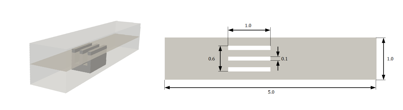
Fig. 118 2D slice of three fin heat sink geometry (All dimensions in \(m\))#
Case Setup#
Note
The python script for this problem can be found at examples/three_fin_2d/heat_sink.py.
Importing the required packages#
In this tutorial you will make use of Channel2D geometry to make the
duct. Line geometry can be used to make inlet, outlet and
intermediate planes for integral boundary conditions. The
AdvectionDiffusion equation is imported from the PDES module.
The parabola and GradNormal are imported from appropriate
modules to generate the required boundary conditions.
# limitations under the License.

import os
import warnings

import torch
import numpy as np
from sympy import Symbol

import physicsnemo.sym
from physicsnemo.sym.hydra import to_absolute_path, instantiate_arch, PhysicsNeMoConfig
from physicsnemo.sym.solver import Solver
from physicsnemo.sym.domain import Domain
from physicsnemo.sym.geometry.primitives_2d import Rectangle, Line, Channel2D
from physicsnemo.sym.utils.sympy.functions import parabola
from physicsnemo.sym.utils.io import csv_to_dict
from physicsnemo.sym.eq.pdes.navier_stokes import NavierStokes, GradNormal
from physicsnemo.sym.eq.pdes.basic import NormalDotVec
from physicsnemo.sym.eq.pdes.turbulence_zero_eq import ZeroEquation
from physicsnemo.sym.eq.pdes.advection_diffusion import AdvectionDiffusion
from physicsnemo.sym.domain.constraint import (
    PointwiseBoundaryConstraint,
    PointwiseInteriorConstraint,
    IntegralBoundaryConstraint,
)
from physicsnemo.sym.domain.monitor import PointwiseMonitor
from physicsnemo.sym.domain.validator import PointwiseValidator
from physicsnemo.sym.key import Key
Creating Geometry#
To generate the geometry of this problem, use
Channel2D for duct and Rectangle for generating the heat sink.
The way of defining Channel2D is same as Rectangle. The
difference between a channel and a rectangle is that a channel is infinite and
composed of only two curves and a rectangle is composed of four curves
that form a closed boundary.
Line is defined using the x and y coordinates of the two endpoints
and the normal direction of the curve. The Line requires
the x coordinates of both the points to be same. A line in arbitrary
orientation can then be created by rotating the Line object.
The following code generates the geometry for the 2D heat sink problem.
def run(cfg: PhysicsNeMoConfig) -> None:
    # params for domain
    channel_length = (-2.5, 2.5)
    channel_width = (-0.5, 0.5)
    heat_sink_origin = (-1, -0.3)
    nr_heat_sink_fins = 3
    gap = 0.15 + 0.1
    heat_sink_length = 1.0
    heat_sink_fin_thickness = 0.1
    inlet_vel = 1.5
    heat_sink_temp = 350
    base_temp = 293.498
    nu = 0.01
    diffusivity = 0.01 / 5

    # define sympy varaibles to parametize domain curves
    _x, y = Symbol("x"), Symbol("y")

    # define geometry
    channel = Channel2D(
        (channel_length[0], channel_width[0]), (channel_length[1], channel_width[1])
    )
    heat_sink = Rectangle(
        heat_sink_origin,
        (
            heat_sink_origin[0] + heat_sink_length,
            heat_sink_origin[1] + heat_sink_fin_thickness,
        ),
    )
    for i in range(1, nr_heat_sink_fins):
        heat_sink_origin = (heat_sink_origin[0], heat_sink_origin[1] + gap)
        fin = Rectangle(
            heat_sink_origin,
            (
                heat_sink_origin[0] + heat_sink_length,
                heat_sink_origin[1] + heat_sink_fin_thickness,
            ),
        )
        heat_sink = heat_sink + fin
    geo = channel - heat_sink

    inlet = Line(
        (channel_length[0], channel_width[0]), (channel_length[0], channel_width[1]), -1
    )
    outlet = Line(
        (channel_length[1], channel_width[0]), (channel_length[1], channel_width[1]), 1
    )

    x_pos = Parameter("x_pos")
    integral_line = Line(
        (x_pos, channel_width[0]),
        (x_pos, channel_width[1]),
        1,
        parameterization=Parameterization({x_pos: channel_length}),
Defining the Equations, Networks and Nodes#
In this problem, you will make two separate network architectures for solving flow and heat variables to achieve increased accuracy.
Additional equations (compared to tutorial Turbulent physics: Zero Equation Turbulence Model)
for imposing Integral continuity (NormalDotVec),
AdvectionDiffusion and GradNormal are specified and the variable to
compute is defined for the GradNormal and AdvectionDiffusion.
Also, it is possible to detach certain variables from the computation
graph in a particular equation if you want to decouple it from
rest of the equations. This uses the .detach() method in the backend
to stop the computation of gradient .
In this
problem, you can stop the gradient calls on \(u\) , \(v\). This
prevents the network from optimizing \(u\) , and \(v\) to
minimize the residual from the advection equation. In this way, you can
make the system one way coupled, where the heat does not influence the
flow, but the flow influences the heat. Decoupling the computations this way can help
the convergence behavior.
    # make list of nodes to unroll graph on
    ze = ZeroEquation(
        nu=nu, rho=1.0, dim=2, max_distance=(channel_width[1] - channel_width[0]) / 2
    )
    ns = NavierStokes(nu=ze.equations["nu"], rho=1.0, dim=2, time=False)
    ade = AdvectionDiffusion(T="c", rho=1.0, D=diffusivity, dim=2, time=False)
    gn_c = GradNormal("c", dim=2, time=False)
    normal_dot_vel = NormalDotVec(["u", "v"])
    flow_net = instantiate_arch(
        input_keys=[Key("x"), Key("y")],
        output_keys=[Key("u"), Key("v"), Key("p")],
        cfg=cfg.arch.fully_connected,
    )
    heat_net = instantiate_arch(
        input_keys=[Key("x"), Key("y")],
        output_keys=[Key("c")],
        cfg=cfg.arch.fully_connected,
    )

    nodes = (
        ns.make_nodes()
        + ze.make_nodes()
        + ade.make_nodes(detach_names=["u", "v"])
        + gn_c.make_nodes()
        + normal_dot_vel.make_nodes()
        + [flow_net.make_node(name="flow_network")]
        + [heat_net.make_node(name="heat_network")]
Setting up the Domain and adding Constraints#
The boundary conditions described in the problem statement are
implemented in the code shown below. Key 'normal_gradient_c' is
used to set the gradient boundary conditions. A new variable
\(c\) is defined for the solving the advection diffusion equation.
In addition to the continuity and Navier-Stokes equations in 2D, you will have to solve the advection diffusion equation (24) (with no source term) in the interior. The thermal diffusivity \(D\) for this problem is 0.002 \(m^2/s\).
You can use integral continuity planes to specify the targeted mass flow rate through these planes.
For a parabolic velocity of 1.5
\(m/s\), the integral mass flow is \(1\) which is added as an
additional constraint to speed up the convergence. Similar to tutorial
Introductory Example you can define keys for 'normal_dot_vel' on
the plane boundaries and set its value to 1 to specify the targeted
mass flow. Use the IntegralBoundaryConstraint constraint to define
these integral constraints. Here the integral_line
geometry was created with a symbolic variable for the line’s x position, x_pos.
The IntegralBoundaryConstraint constraint will randomly generate samples
for various x_pos values. The number of such samples can be controlled by batch_size argument,
while the points in each sample can be configured by integral_batch_size argument.
The range for the symbolic variables (in this case x_pos) can be set using the parameterization argument.
These planes (lines for 2D geometry) would then be used when
the NormalDotVec PDE that will compute the dot product of normal components of the
geometry and the velocity components. The parabolic profile can be created by using the parabola function
by specifying the variable for sweep, the two intercepts and max height.
    # make domain
    domain = Domain()

    # inlet
    inlet_parabola = parabola(
        y, inter_1=channel_width[0], inter_2=channel_width[1], height=inlet_vel
    )
    inlet = PointwiseBoundaryConstraint(
        nodes=nodes,
        geometry=inlet,
        outvar={"u": inlet_parabola, "v": 0, "c": 0},
        batch_size=cfg.batch_size.inlet,
    )
    domain.add_constraint(inlet, "inlet")

    # outlet
    outlet = PointwiseBoundaryConstraint(
        nodes=nodes,
        geometry=outlet,
        outvar={"p": 0},
        batch_size=cfg.batch_size.outlet,
    )
    domain.add_constraint(outlet, "outlet")

    # heat_sink wall
    hs_wall = PointwiseBoundaryConstraint(
        nodes=nodes,
        geometry=heat_sink,
        outvar={"u": 0, "v": 0, "c": (heat_sink_temp - base_temp) / 273.15},
        batch_size=cfg.batch_size.hs_wall,
    )
    domain.add_constraint(hs_wall, "heat_sink_wall")

    # channel wall
    channel_wall = PointwiseBoundaryConstraint(
        nodes=nodes,
        geometry=channel,
        outvar={"u": 0, "v": 0, "normal_gradient_c": 0},
        batch_size=cfg.batch_size.channel_wall,
    )
    domain.add_constraint(channel_wall, "channel_wall")

    # interior flow
    interior_flow = PointwiseInteriorConstraint(
        nodes=nodes,
        geometry=geo,
        outvar={"continuity": 0, "momentum_x": 0, "momentum_y": 0},
        batch_size=cfg.batch_size.interior_flow,
        compute_sdf_derivatives=True,
        lambda_weighting={
            "continuity": Symbol("sdf"),
            "momentum_x": Symbol("sdf"),
            "momentum_y": Symbol("sdf"),
        },
    )
    domain.add_constraint(interior_flow, "interior_flow")

    # interior heat
    interior_heat = PointwiseInteriorConstraint(
        nodes=nodes,
        geometry=geo,
        outvar={"advection_diffusion_c": 0},
        batch_size=cfg.batch_size.interior_heat,
        lambda_weighting={
            "advection_diffusion_c": 1.0,
        },
    )
    domain.add_constraint(interior_heat, "interior_heat")

    # integral continuity
    def integral_criteria(invar, params):
        sdf = geo.sdf(invar, params)
        return np.greater(sdf["sdf"], 0)

    integral_continuity = IntegralBoundaryConstraint(
        nodes=nodes,
        geometry=integral_line,
        outvar={"normal_dot_vel": 1},
        batch_size=cfg.batch_size.num_integral_continuity,
        integral_batch_size=cfg.batch_size.integral_continuity,
        lambda_weighting={"normal_dot_vel": 0.1},
        criteria=integral_criteria,
    )
Adding Monitors and Validators#
The validation data comes from a 2D simulation computed using OpenFOAM and the code to import it can be found below.
    # add validation data
    file_path = "openfoam/heat_sink_zeroEq_Pr5_mesh20.csv"
    if os.path.exists(to_absolute_path(file_path)):
        mapping = {
            "Points:0": "x",
            "Points:1": "y",
            "U:0": "u",
            "U:1": "v",
            "p": "p",
            "d": "sdf",
            "nuT": "nu",
            "T": "c",
        }
        openfoam_var = csv_to_dict(to_absolute_path(file_path), mapping)
        openfoam_var["nu"] += nu
        openfoam_var["c"] += -base_temp
        openfoam_var["c"] /= 273.15
        openfoam_invar_numpy = {
            key: value
            for key, value in openfoam_var.items()
            if key in ["x", "y", "sdf"]
        }
        openfoam_outvar_numpy = {
            key: value
            for key, value in openfoam_var.items()
            if key in ["u", "v", "p", "c"]  # Removing "nu"
        }
        openfoam_validator = PointwiseValidator(
            nodes=nodes,
            invar=openfoam_invar_numpy,
            true_outvar=openfoam_outvar_numpy,
        )
        domain.add_validator(openfoam_validator)
    else:
        warnings.warn(
            f"Directory {file_path} does not exist. Will skip adding validators. Please download the additional files from NGC https://catalog.ngc.nvidia.com/orgs/nvidia/teams/physicsnemo/resources/physicsnemo_sym_examples_supplemental_materials"
        )

    # monitors for force, residuals and temperature
    global_monitor = PointwiseMonitor(
        geo.sample_interior(100),
        output_names=["continuity", "momentum_x", "momentum_y"],
        metrics={
            "mass_imbalance": lambda var: torch.sum(
                var["area"] * torch.abs(var["continuity"])
            ),
            "momentum_imbalance": lambda var: torch.sum(
                var["area"]
                * (torch.abs(var["momentum_x"]) + torch.abs(var["momentum_y"]))
            ),
        },
        nodes=nodes,
        requires_grad=True,
    )
    domain.add_monitor(global_monitor)

    force = PointwiseMonitor(
        heat_sink.sample_boundary(100),
        output_names=["p"],
        metrics={
            "force_x": lambda var: torch.sum(var["normal_x"] * var["area"] * var["p"]),
            "force_y": lambda var: torch.sum(var["normal_y"] * var["area"] * var["p"]),
        },
        nodes=nodes,
    )
    domain.add_monitor(force)

    peakT = PointwiseMonitor(
        heat_sink.sample_boundary(100),
        output_names=["c"],
        metrics={"peakT": lambda var: torch.max(var["c"])},
        nodes=nodes,
    )
Training the model#
Once the python file is setup, the training can be started by executing the python script.
python heat_sink.py
Results and Post-processing#
The results for the PhysicsNeMo Sym simulation are compared against the OpenFOAM data in Fig. 119.
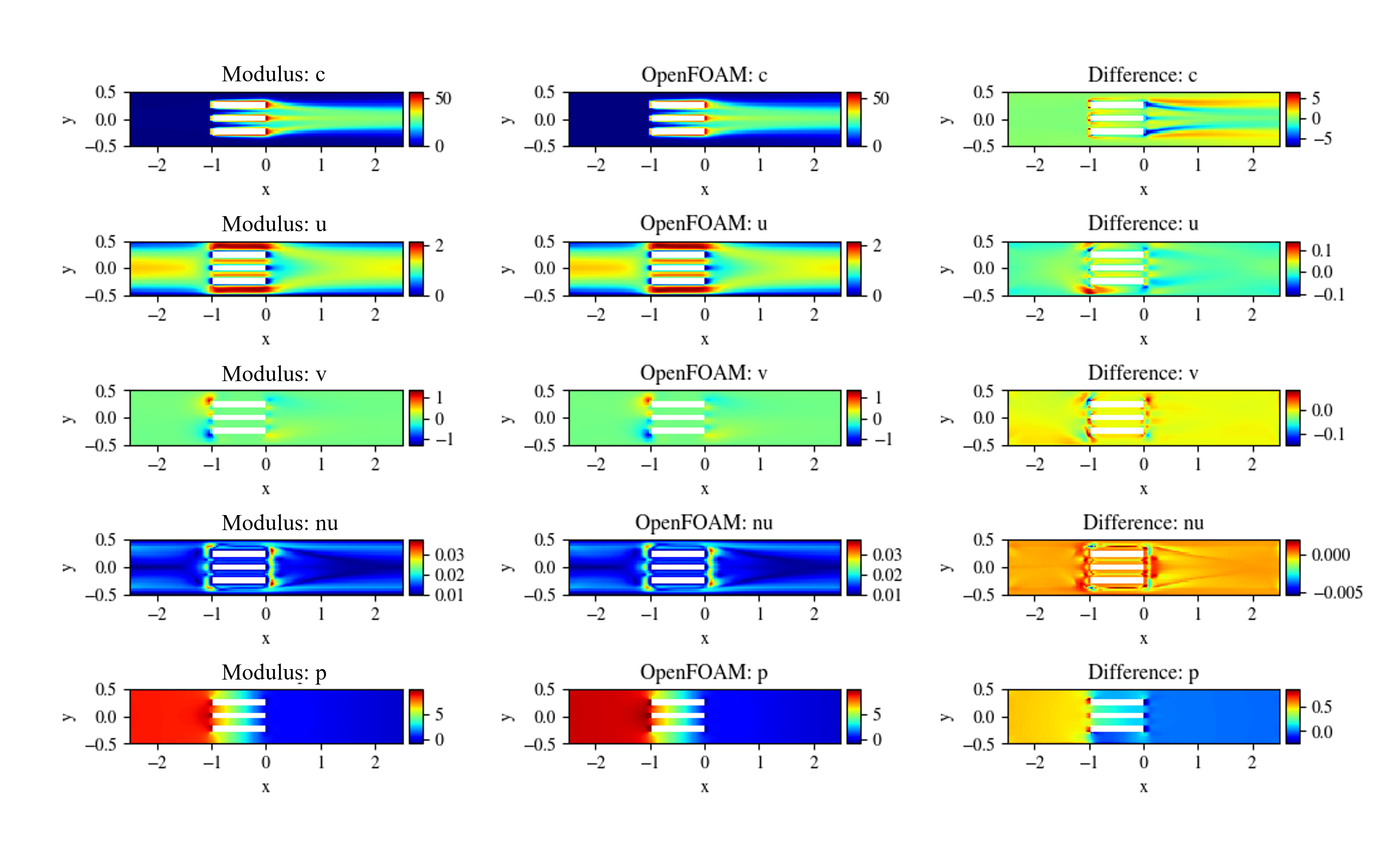
Fig. 119 Left: PhysicsNeMo Sym. Center: OpenFOAM. Right: Difference#