Parameterized 3D Heat Sink#
Introduction#
This tutorial walks through the process of simulating a parameterized problem using PhysicsNeMo Sym. The neural networks in PhysicsNeMo Sym allow us to solve problems for multiple parameters/independent variables in a single training. These parameters can be geometry variables, coefficients of a PDE or even boundary conditions. Once the training is complete, it is possible to run inference on several geometry/physical parameter combinations as a post-processing step, without solving the forward problem again. You will see that such parameterization increases the computational cost only fractionally while solving the entire desired design space.
To demonstrate this feature, this example will solve the flow and heat over a 3-fin heat sink whose fin height, fin thickness, and fin length are variable. We will then perform a design optimization to find out the most optimal fin configuration for the heat sink example. By the end of this tutorial, you would learn to easily convert any simulation to a parametric design study using PhysicsNeMo Sym’s CSG module and Neural Network solver. In this tutorial, you would learn the following:
How to set up a parametric simulation in PhysicsNeMo Sym.
Note
This tutorial is an extension of tutorial Conjugate Heat Transfer which discussed how to use PhysicsNeMo Sym for solving Conjugate Heat problems. This tutorial uses the same geometry setup and solves it for a parameterized setup at an increased Reynolds number. Hence, it is recommended that you to refer tutorial Conjugate Heat Transfer for any additional details related to geometry specification and boundary conditions.
The same scripts used in example Conjugate Heat Transfer will be used. To make the simulation parameterized and turbulent, you will set the custom flags parameterized and turbulent both as true in the config files.
Note
In this tutorial the focus will be on parameterization which is independent of the physics being solved and can be applied to any class of problems covered in the User Guide.
Problem Description#
Please refer the geometry and boundary conditions for a 3-fin heat sink in tutorial Conjugate Heat Transfer. We will parameterize this problem to solve for several heat sink designs in a single neural network training. We will modify the heat sink’s fin dimensions (thickness, length and height) to create a design space of various heat sinks. The Re for this case is now 500 and you will incorporate turbulence using Zero Equation turbulence model.
For this problem, you will vary the height (\(h\)), length (\(l\)), and thickness (\(t\)) of the central fin and the two side fins. The height, length, and thickness of the two side fins are kept the same, and therefore, there will be a total of six geometry parameters. The ranges of variation for these geometry parameters are given in equation (41).
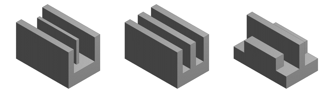
Fig. 193 Examples of some of the 3 Fin geometries covered in the chosen design space#
Case Setup#
In this tutorial, you will use the 3D geometry module from PhysicsNeMo Sym to create the parameterized 3-fin heat sink geometry. Discrete parameterization can sometimes lead to discontinuities in the solution making the training harder. Hence tutorial only covers parameters that are continuous. Also, you will be training the parameterized model and validating it by performing inference on a case where \(h_{central fin}=0.4\), \(h_{side fins}=0.4\), \(l_{central fin}=1.0\), \(l_{side fins}=1.0\), \(t_{central fin}=0.1\), and \(t_{side fins}=0.1\). At the end of the tutorial a comparison between results for the above combination of parameters obtained from a parameterized model versus results obtained from a non-parameterized model trained on just a single geometry corresponding to the same set of values is presented. This will highlight the usefulness of using PINNs for doing parameterized simulations in comparison to some of the traditional methods.
Since the majority of the problem definition and setup was covered in Conjugate Heat Transfer, this tutorial will focus only on important elements for the parameterization.
Creating Nodes and Architecture for Parameterized Problems#
The parameters chosen for variables act as additional inputs to the neural network. The outputs remain the same. Also, for this example since the variables are geometric only, no change needs to be made for how the equation nodes are defined (except the addition of turbulence model). In cases where the coefficients of a PDE are parameterized, the corresponding coefficient needs to be defined symbolically (i.e. using string) in the equation node.
Note for this example, the viscosity is set as a string in the NavierStokes constructor for the purposes of turbulence model. The ZeroEquation equation node 'nu' as the output node which acts as input to the momentum equations in Navier-Stokes.
The code for this parameterized problem is shown below. Note that parameterized and turbulent are set to true in the config file.
Parameterized flow network:
        ns = NavierStokes(nu=ze.equations["nu"], rho=1.0, dim=3, time=False)
        navier_stokes_nodes = ns.make_nodes() + ze.make_nodes()
    else:
        ns = NavierStokes(nu=0.01, rho=1.0, dim=3, time=False)
        navier_stokes_nodes = ns.make_nodes()
    normal_dot_vel = NormalDotVec()

    # make network arch
    if cfg.custom.parameterized:
        input_keys = [
            Key("x"),
            Key("y"),
            Key("z"),
            Key("fin_height_m"),
            Key("fin_height_s"),
            Key("fin_length_m"),
            Key("fin_length_s"),
            Key("fin_thickness_m"),
            Key("fin_thickness_s"),
        ]
    else:
        input_keys = [Key("x"), Key("y"), Key("z")]
    flow_net = FullyConnectedArch(
        input_keys=input_keys, output_keys=[Key("u"), Key("v"), Key("w"), Key("p")]
    )

    # make list of nodes to unroll graph on
    flow_nodes = (
        navier_stokes_nodes
        + normal_dot_vel.make_nodes()
        + [flow_net.make_node(name="flow_network")]
    )

    geo = ThreeFin(parameterized=cfg.custom.parameterized)

    # params for simulation
Parameterized heat network:
    dif_inteface = DiffusionInterface("theta_f", "theta_s", 1.0, 5.0, dim=3, time=False)
    f_grad = GradNormal("theta_f", dim=3, time=False)
    s_grad = GradNormal("theta_s", dim=3, time=False)

    # make network arch
    if cfg.custom.parameterized:
        input_keys = [
            Key("x"),
            Key("y"),
            Key("z"),
            Key("fin_height_m"),
            Key("fin_height_s"),
            Key("fin_length_m"),
            Key("fin_length_s"),
            Key("fin_thickness_m"),
            Key("fin_thickness_s"),
        ]
    else:
        input_keys = [Key("x"), Key("y"), Key("z")]
    flow_net = FullyConnectedArch(
        input_keys=input_keys,
        output_keys=[Key("u"), Key("v"), Key("w"), Key("p")],
    )
    thermal_f_net = FullyConnectedArch(
        input_keys=input_keys, output_keys=[Key("theta_f")]
    )
    thermal_s_net = FullyConnectedArch(
        input_keys=input_keys, output_keys=[Key("theta_s")]
    )

    # make list of nodes to unroll graph on
    thermal_nodes = (
        ad.make_nodes()
        + dif.make_nodes()
        + dif_inteface.make_nodes()
        + f_grad.make_nodes()
        + s_grad.make_nodes()
        + [flow_net.make_node(name="flow_network", optimize=False)]
        + [thermal_f_net.make_node(name="thermal_f_network")]
        + [thermal_s_net.make_node(name="thermal_s_network")]
    )

    geo = ThreeFin(parameterized=cfg.custom.parameterized)

    # params for simulation
Setting up Domain and Constraints#
This section is again very similar to Conjugate Heat Transfer tutorial. The only difference being, now
the input to parameterization argument is a dictionary of key value pairs where the keys are strings for each design variable and the values are tuples of float/ints specifying the range of variation for those variables.
The code to setup these dictionaries for parameterized inputs and constraints can be found below.
Setting the parameter ranges (three_fin_geometry.py)
height_s_range = (0.0, 0.6)
length_m_range = (0.5, 1.0)
length_s_range = (0.5, 1.0)
thickness_m_range = (0.05, 0.15)
thickness_s_range = (0.05, 0.15)
param_ranges = {
    fin_height_m: height_m_range,
    fin_height_s: height_s_range,
    fin_length_m: length_m_range,
    fin_length_s: length_s_range,
    fin_thickness_m: thickness_m_range,
    fin_thickness_s: thickness_s_range,
}
fixed_param_ranges = {
    fin_height_m: 0.4,
    fin_height_s: 0.4,
    fin_length_m: 1.0,
    fin_length_s: 1.0,
    fin_thickness_m: 0.1,
    fin_thickness_s: 0.1,
}

# geometry params for domain
channel_origin = (-2.5, -0.5, -0.5)
channel_dim = (5.0, 1.0, 1.0)
heat_sink_base_origin = (-1.0, -0.5, -0.3)
heat_sink_base_dim = (1.0, 0.2, 0.6)
            pr = Parameterization(param_ranges)
            self.pr = param_ranges
        else:
            pr = Parameterization(fixed_param_ranges)
            self.pr = fixed_param_ranges

        # channel
        self.channel = Channel(
            channel_origin,
            (
                channel_origin[0] + channel_dim[0],
                channel_origin[1] + channel_dim[1],
                channel_origin[2] + channel_dim[2],
            ),
            parameterization=pr,
        )

        # three fin heat sink
        heat_sink_base = Box(
            heat_sink_base_origin,
            (
                heat_sink_base_origin[0] + heat_sink_base_dim[0],  # base of heat sink
Setting the parameterization argument in the constraints.
Here, only a few BCs from the flow domain are shown for example purposes.
But the same settings are applied to all the other BCs.
        nodes=flow_nodes,
        geometry=geo.inlet,
        outvar={"u": u_profile, "v": 0, "w": 0},
        batch_size=cfg.batch_size.Inlet,
        criteria=Eq(x, channel_origin[0]),
        lambda_weighting={
            "u": 1.0,
            "v": 1.0,
            "w": 1.0,
        },  # weight zero on edges
        parameterization=geo.pr,
        batch_per_epoch=5000,
    )
    flow_domain.add_constraint(constraint_inlet, "inlet")

    # outlet
    constraint_outlet = PointwiseBoundaryConstraint(
        return np.greater(sdf["sdf"], 0)

    integral_continuity = IntegralBoundaryConstraint(
        nodes=flow_nodes,
        geometry=geo.integral_plane,
        outvar={"normal_dot_vel": volumetric_flow},
        batch_size=5,
        integral_batch_size=cfg.batch_size.IntegralContinuity,
        criteria=integral_criteria,
        lambda_weighting={"normal_dot_vel": 1.0},
        parameterization={**geo.pr, **{x_pos: (-1.1, 0.1)}},
        fixed_dataset=False,
        num_workers=4,
    )
    flow_domain.add_constraint(integral_continuity, "integral_continuity")

    # flow data
    file_path = "../openfoam/"
    if os.path.exists(to_absolute_path(file_path)):
Training the Model#
This part is exactly similar to tutorial Conjugate Heat Transfer and once all the definitions are complete, you can execute the parameterized problem like any other problem.
Design Optimization#
As discussed previously, you can optimize the design once the training is complete as a post-processing step. A typical design optimization usually contains an objective function that is minimized/maximized subject to some physical/design constraints.
For heat sink designs, usually the peak temperature that can be reached at the source chip is limited. This limit arises from the operating temperature requirements of the chip on which the heat sink is mounted for cooling purposes. The design is then constrained by the maximum pressure drop that can be successfully provided by the cooling system that pushes the flow around the heat sink. Mathematically this can be expressed as below:
Variable/Function |
Description |
|
minimize |
\(Peak \text{ } Temperature\) |
Minimize the peak temperature at the source chip |
with respect to |
\(h_{central fin}, h_{side fins}, l_{central fin}, l_{side fins}, t_{central fin}, t_{side fins}\) |
Geometric Design variables of the heat sink |
subject to |
\(Pressure \text{ } drop < 2.5\) |
Limit on the pressure drop (Max pressure drop that can be provided by cooling system |
Such optimization problems can be easily achieved in PhysicsNeMo Sym once you have a trained, parameterized model ready.
As it can be noticed, while solving the parameterized simulation you
created some monitors to track the peak temperature and the pressure
drop for some design variable combination. You will basically would follow the
same process and use the PointwiseMonitor constructor to find the values for
multiple combinations of the design variables. You can create
this simply by looping through the multiple designs. Since these monitors can be for large number of design variable combinations, you are recommended to use these
monitors only after the training is complete to achieve better
computational efficiency. Do do this, once the models are trained, you can run the flow and thermal models in the 'eval' mode by specifying: 'run_mode=eval'
in the config files.
After the models are run in the 'eval' mode, the pressure drop and peak temperature values will be saved in form of a .csv file. Then,
one can write a simple scripts to sift through the various samples and pick the most optimal ones that minimize/maximize the objective function while meeting the
required constraints (for this example, the design with the least peak temperature and the maximum pressure drop < 2.5):
# SPDX-FileCopyrightText: Copyright (c) 2023 - 2024 NVIDIA CORPORATION & AFFILIATES.
# SPDX-FileCopyrightText: All rights reserved.
# SPDX-License-Identifier: Apache-2.0
#
# Licensed under the Apache License, Version 2.0 (the "License");
# you may not use this file except in compliance with the License.
# You may obtain a copy of the License at
#
#     http://www.apache.org/licenses/LICENSE-2.0
#
# Unless required by applicable law or agreed to in writing, software
# distributed under the License is distributed on an "AS IS" BASIS,
# WITHOUT WARRANTIES OR CONDITIONS OF ANY KIND, either express or implied.
# See the License for the specific language governing permissions and
# limitations under the License.

"""
NOTE: run three_fin_flow and Three_fin_thermal in "eval" mode
after training to get the monitor values for different designs.
"""

# import PhysicsNeMo library
from physicsnemo.sym.utils.io.csv_rw import dict_to_csv
from physicsnemo.sym.hydra import to_absolute_path

# import other libraries
import numpy as np
import os
import sys
import csv

# specify the design optimization requirements
max_pressure_drop = 2.5
num_design = 10
path_flow = to_absolute_path("outputs/run_mode=eval/three_fin_flow")
path_thermal = to_absolute_path("outputs/run_mode=eval/three_fin_thermal")
invar_mapping = [
    "fin_height_middle",
    "fin_height_sides",
    "fin_length_middle",
    "fin_length_sides",
    "fin_thickness_middle",
    "fin_thickness_sides",
]
outvar_mapping = ["pressure_drop", "peak_temp"]


# read the monitor files, and perform a design space search
def DesignOpt(
    path_flow,
    path_thermal,
    num_design,
    max_pressure_drop,
    invar_mapping,
    outvar_mapping,
):
    path_flow += "/monitors"
    path_thermal += "/monitors"
    directory = os.path.join(os.getcwd(), path_flow)
    sys.path.append(path_flow)
    values, configs = [], []

    for _, _, files in os.walk(directory):
        for file in files:
            if file.startswith("back_pressure") & file.endswith(".csv"):
                value = []
                configs.append(file[13:-4])

                # read back pressure
                with open(os.path.join(path_flow, file), "r") as datafile:
                    data = []
                    reader = csv.reader(datafile, delimiter=",")
                    for row in reader:
                        columns = [row[1]]
                        data.append(columns)
                    last_row = float(data[-1][0])
                    value.append(last_row)

                # read front pressure
                with open(
                    os.path.join(path_flow, "front_pressure" + file[13:]), "r"
                ) as datafile:
                    reader = csv.reader(datafile, delimiter=",")
                    data = []
                    for row in reader:
                        columns = [row[1]]
                        data.append(columns)
                    last_row = float(data[-1][0])
                    value.append(last_row)

                # read temperature
                with open(
                    os.path.join(path_thermal, "peak_temp" + file[13:]), "r"
                ) as datafile:
                    data = []
                    reader = csv.reader(datafile, delimiter=",")
                    for row in reader:
                        columns = [row[1]]
                        data.append(columns)
                    last_row = float(data[-1][0])
                    value.append(last_row)
                values.append(value)

    # perform the design optimization
    values = np.array(
        [
            [values[i][1] - values[i][0], values[i][2] * 273.15]
            for i in range(len(values))
        ]
    )
    indices = np.where(values[:, 0] < max_pressure_drop)[0]
    values = values[indices]
    configs = [configs[i] for i in indices]
    opt_design_index = values[:, 1].argsort()[0:num_design]
    opt_design_values = values[opt_design_index]
    opt_design_configs = [configs[i] for i in opt_design_index]

    # Save to a csv file
    opt_design_configs = np.array(
        [
            np.array(opt_design_configs[i][1:].split("_")).astype(float)
            for i in range(num_design)
        ]
    )
    opt_design_configs_dict = {
        key: value.reshape(-1, 1)
        for (key, value) in zip(invar_mapping, opt_design_configs.T)
    }
    opt_design_values_dict = {
        key: value.reshape(-1, 1)
        for (key, value) in zip(outvar_mapping, opt_design_values.T)
    }
    opt_design = {**opt_design_configs_dict, **opt_design_values_dict}
    dict_to_csv(opt_design, "optimal_design")
    print("Finished design optimization!")


if __name__ == "__main__":
    DesignOpt(
        path_flow,
        path_thermal,
        num_design,
        max_pressure_drop,
        invar_mapping,
        outvar_mapping,
    )
Results#
The design parameters for the optimal heat sink for this problem are: \(h_{central fin} = 0.4\), \(h_{side fins} = 0.4\), \(l_{central fin} = 0.83\), \(l_{side fins} = 1.0\), \(t_{central fin} = 0.15\), \(t_{side fins} = 0.15\). The above design has a pressure drop of 2.46 and a peak temperature of 76.23 \((^{\circ} C)\) Fig. 194
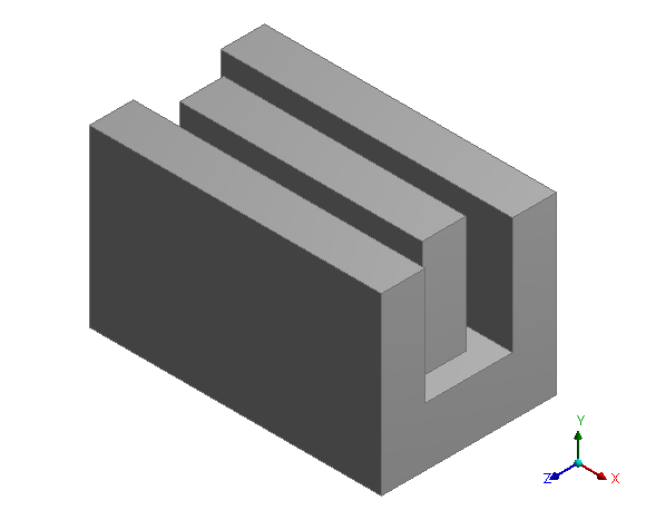
Fig. 194 Three Fin geometry after optimization#
Table 14 represents the computed pressure drop and peak temperature for the OpenFOAM single geometry and PhysicsNeMo Sym single and parameterized geometry runs. It is evident that the results for the parameterized model are close to those of a single geometry model, showing its good accuracy.
Property |
OpenFOAM Single Run |
Single Run |
Parameterized Run |
Pressure Drop \((Pa)\) |
2.195 |
2.063 |
2.016 |
Peak Temperature \((^{\circ} C)\) |
72.68 |
76.10 |
77.41 |
By parameterizing the geometry, PhysicsNeMo Sym significantly accelerates design optimization when compared to traditional solvers, which are limited to single geometry simulations. For instance, 3 values (two end values of the range and a middle value) per design variable would result in \(3^6 = 729\) single geometry runs. The total compute time required by OpenFOAM for this design optimization would be 4099 hrs. (on 20 processors). PhysicsNeMo Sym can achieve the same design optimization at ~17x lower computational cost. Large number of design variables or their values would only magnify the difference in the time taken for two approaches.
Note
The PhysicsNeMo Sym calculations were done using 4 NVIDIA V100 GPUs. The OpenFOAM calculations were done using 20 processors.
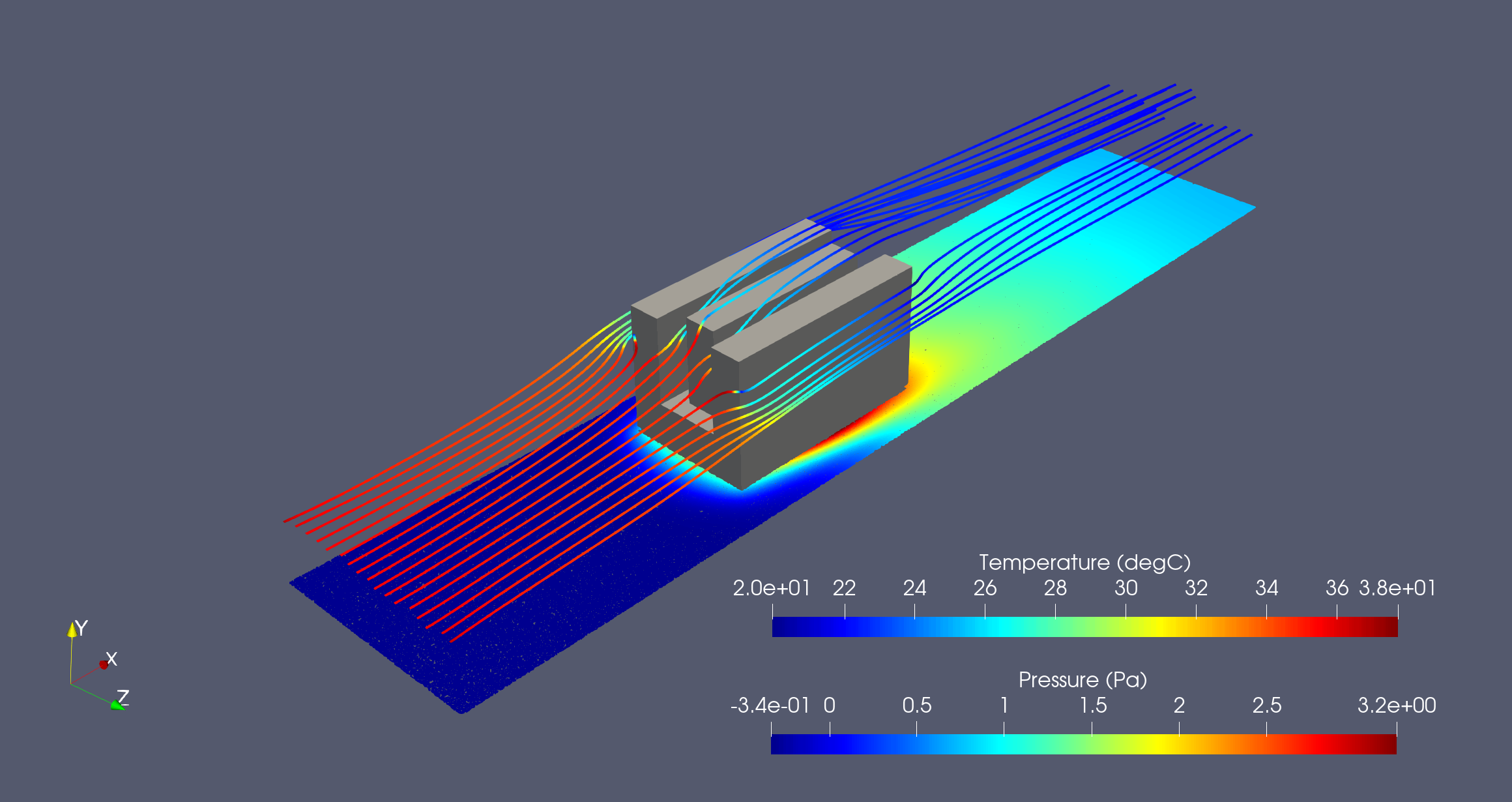
Fig. 195 Streamlines colored with pressure and temperature profile in the fluid for optimal three fin geometry#
Here, the 3-Fin heatsink was solved for arbitrary heat properties chosen such that the coupled conjugate heat transfer solution was possible. However, such approach causes issues when the conductivities are orders of magnitude different at the interface. We will revisit the conjugate heat transfer problem in tutorial Heat Transfer with High Thermal Conductivity and Industrial Heat Sink to see some advanced tricks/schemes that one can use to handle the issues that arise in Neural network training when real material properties are involved.