Diffusion Model for Full-Waveform Inversion (FWI)#
Problem Overview#
In the context of geophysics, Full Waveform Inversion (FWI) is a seismic imaging technique that reconstructs subsurface properties, also called velocity model, by fitting the recorded seismic waveform. It underpins a range of applications, including:
Hydro-carbon exploration and production, where an accurate velocity model guides drilling decisions.
CO₂ storage, ensuring the integrity of underground reservoirs used for carbon capture and sequestration.
Global and regional seismology, helping characterise tectonic processes and earthquakes.
Analogous elastic/acoustic imaging modalities such as medical ultrasound and non-destructive testing.
The present example is tailored to the elastic wave equation in the context of hydro-carbon exploration, but the same framework can be applied to other wave equations and applications.
The following introduces a few key concepts that are essential to FWI in the context of hydro-carbon exploration:
Velocity model \(\mathbf{x}(r)=\bigl[ V_\mathrm{P},\,V_\mathrm{S},\,\rho \bigr]\) – a 3-D image over coordinates \(r = (z,x,y)\), where \(z\) is the depth, and \(x\) and \(y\) are the surface coordinates. The P-wave velocity is denoted by \(V_\mathrm{P}\), the S-wave velocity by \(V_\mathrm{S}\), and \(\rho\) is the density. The velocity model spans several kilometres and is discretised at metre-scale resolution.
Sources / shots – positions \(r_s = (0, x_s, y_s)_{1 \leq s \leq S}\) where independent excitations are fired; typically thousands of shots distributed along the surface. The cost associated with acquiring these shots and processing the data is a major component of the total cost of the FWI.
Receivers – sensors at locations \(r_i = (0, x_i, y_i)_{1 \leq i \leq R}\) that record horizontal particle-velocity components \(v_x\) and \(v_y\) and vertical particle-velocity component \(v_z\) at the surface. Receivers are typically arranged in a 2-D grid of \(\mathcal{O}(10^3)\) sensors with a few-meter spacing and record data with a time-resolution of a few tenth of seconds.
Seismic observations - the particle-velocity components recorded at all receivers for a given shot \(s\) can be combined into a 3D image \(y_s = [v_z, v_x, v_y]\) over coordinates \((t, x_i, y_i)\) that contains reflections, refractions and surface waves. The \(S\) independent sources can be further combined to form a large set \(\mathbf{y}\) of 3D observations.
The goal of FWI is to reconstruct the velocity model \(\mathbf{x}(r)\) from the entire set of seismic observations \(\mathbf{y}\). To do so, standard FWI uses classical optimization techniques combined with the elastic wave equation, defined in Equation (1) below.
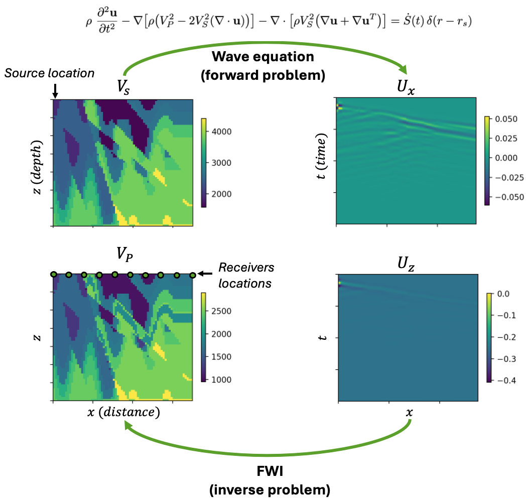
Fig. 54 Introduction to FWI#
where \(\dot{S}(t)\delta(r-r_s)\) is the source at location \(r_s\) with time signal \(\dot{S}(t)\), and \(\mathcal{A}_{\mathbf{x}}\) is the elastic wave operator defined by:
We denote \(\mathcal{R} (\mathbf{x}, s)\) the solution operator associated to the wave equation \((1)\). This operator maps a velocity model \(\mathbf{x}\) and a source \(\dot{S}(t)\delta(r-r_s)\) to the solution of the PDE at the receiver locations: it therefore provides a simulated seismic observation \(\hat{y}_s\).
FWI seeks to solve an inverse problem of finding the velocity model \(\mathbf{x}\) that best fits the observed seismic data \(\mathbf{y}\). Given observed data, standard FWI uses classical optimization techniques to solve the following minimization problem:
In realistic conditions (limited number of observations, limited resolution, noise), the inverse problem defined by this equation is ill-posed (that is, it has multiple solutions). This one-to-many mapping is the main difficulty of FWI and makes it particularly suitable to be solved with generative models. This example uses a diffusion model to solve the FWI inverse problem.
Prerequisites#
This example requires basic knowledge of denoising diffusion models; it is also recommended to be familiar with other examples using diffusion models, such as StormCast or CorrDiff.
Start by installing PhysicsNeMo (if not already installed) and copying this folder (examples/geophysics/diffusion_fwi) to a system with a GPU available.
Then, install the required dependencies by running below:
pip install -r requirements.txt
or, if you need fine-grained control over the dependencies, you can install them individually:
pip install hydra-core>=1.2.0 omegaconf>=2.3.0 wandb>=0.13.7 deepwave>=0.0.21
Note that the deepwave dependency is only necessary for generating the dataset and for physics-informed sampling. For data download and processing, it is also required to have zip and unzip installed. As those may not be shipped in the currentb physicsnemo container, you may need to install them manually. For example, on Ubuntu, you can run:
sudo apt update
sudo apt-get install zip unzip
This example comprises a succession of three steps, detailed below:
Dataset Preprocessing#
This examples builds on the E-FWI dataset, initially published as E-FWI: Multi-parameter Benchmark Datasets for Elastic Full Waveform Inversion of Geophysical Properties. We complement the original dataset by providing a data generation pipeline to:
expand the dataset to the case of variable density \(\rho(r)\)
generate particle-velocity observations from veloicty models in a consistent manner
⚠️ Warning: The E-FWI dataset is distributed under a non-commercial license CC BY-NC-SA 4.0.
Step 1: Download and Reorganize the E-FWI Dataset#
The first step is to download the E-FWI dataset. Because the E-FWI dataset is composed of multiple sub-datasets (CFB, CFA, FVB), we provide utility functions to merge them into a single dataset and reorganize the data into a more convenient format.
To pre-process the entire dataset, navigate to the ./data directory and run:
python download_data.py --download --reorganize --clean --shuffle --name all
This will download the dataset as a collection of .npz files in the directory ./data/all/samples. For more information about the possible options, run:
python download_data.py --help
Note: Depending on how many subsets of the E-FWI dataset you want to download, the size of the dataset can be quite large (from 100GB to 1TB); downloading the full dataset can take several hours.
Step 2: Generate Seismic Observations#
The second step consists in re-generating seismic observations from the velocity models with variable density. The original wave speeds \(V_\mathrm{P}\) and \(V_\mathrm{S}\) from the E-FWI datasets are retained and the density is generated by the generate_data.py script. This script then solve an elastic wave equation using Deepwave to generate the seismic observations. Because this step can be time-consuming, it is advised to do it on a machine with multiple GPUs. To do so, still in the ./data directory run:
python generate_data.py --in_dir ./all --out_dir <path_to_output_directory>
This script will generate a new set of .npz files in the directory <path_to_output_directory>/samples.
A useful option is to specify the frequency of the source signal, which can be done by passing the --source_frequency <frequency> option to the generate_data.py script. The default frequency is 15 Hz. This value correspond to the peak frequency of the Ricker wavelet used to generate the source signal.
Step 3: Compute Dataset Statistics#
For the dataset preprocessing, compute statistics of the train and test sets by running:
python compute_stats.py --dir <path_to_output_directory> --batch_size 512 --num_workers 4
This script will compute the dataset statistics and save them in the file <path_to_output_directory>/stats.json. It supports distributed processing based on torch.distributed, so it is advised to run it on a machine with multiple GPUs. If doing so, replace the python command with:
torchrun --standalone --nnodes=<NUM_NODES> --nproc_per_node=<NUM_GPUS_PER_NODE> compute_stats.py --dir <path_to_output_directory> --batch_size 512 --num_workers 4
After these steps are completed, verify that you have a dataset ready to be used for training.
Training#
Configuration Basics
Training is handled by
train.py, configured using Hydra based on the contents of theconfigdirectory. Hydra allows for YAML-based modular and hierarchical configuration management and supports command-line overrides for rapid testing and experimentation. Theconf/config_train.yamlfile includes the default parameters for training a diffusion model for FWI. It contains some fields that must be provided by the user at runtime. This can be done by directly editing theconf/config_train.yamlfile (or a copy of it), or by using hydra overrides.
To train the model with a specific dataset and set a non-default batch size, one can run:
python train.py --config-name=config_train ++dataset.directory=<path_to_dataset_directory> ++training.batch_size_per_device=1024
At runtime, Hydra will parse the config subdirectory and command line overrides into a runtime configuration object cfg, which will have all settings accessible through both attribute or dictionary-like interfaces. For example, the batch size per device can be accessed either as cfg.training.batch_size_per_device or cfg['training']['batch_size_per_device'].
The training script train.py will initialize the training experiment and launch the main training loop.
If running on a machine (single node) with multiple GPUs, the training script can be parallelized with Distributed Data Parallel (DDP). To do so, run:
torchrun --standalone --nnodes=1 --nproc_per_node=<NUM_GPUS_PER_NODE> train.py --config-name=config_train ++dataset.directory=<path_to_dataset_directory> ++training.batch_size_per_device=1024
To train on multiple nodes or multiple machines, this command needs to be modified and it is recommended to refer to the torchrun documentation.
The training script should produce multiple outputs:
Training logs containing loss values and runtime statistics, either in the console or in the directory
./outputsCheckpoints saved in the directory specified by
++io.checkpoint_dir=<path_to_checkpoint_directory>. This contains the trained model checkpoints for inference, as well as checkpoints for resuming training.If required, Weights & Biases logs saved in the directory specified by
++wandb.results_dir=<path_to_wandb_directory>.
Sampling and Model Evaluation#
After training the model, it can be used to generate samples from the learned distribution \(p(\mathbf{x} | \mathbf{y})\) over the velocity model \(\mathbf{x}\) and conditioned on the observed seismic data \(\mathbf{y}\). This is handled by the generate.py script, which also relies on a hydra-based configuration in the conf/config_generate.yaml file. This example supports two types of sampling:
Zero-shot sampling - purely data-driven approaches that only uses the learned distribution \(p(\mathbf{x} | \mathbf{y})\).
Physics-informed sampling - utilizes Diffusion Posterior Sampling (DPS) with a physics-informed guidance term that enforces consistency between the PDE residuals (Eq. 1) and the observed data.
Zero-Shot Sampling#
To generate samples from the learned distribution \(p(\mathbf{x} | \mathbf{y})\), one needs to solve the reverse diffusion process defined the following SDE:
In this equation, \(t\) is the diffusion time, and \(\mathbf{f}\) and \(g\) are the drift and diffusion terms, respectively. \(\nabla_x \log p_t(\mathbf{x}_t | \mathbf{y})\) is the conditional score function previously learned during training, and \(\mathbf{w}_t\) is a standard Wiener process. In this example, we adopt the EDM framework to solve this SDE and generate clean samples \(\mathbf{x}_0\) from noisy latent state \(\mathbf{x}_T\).
The generate.py script implements this sampling procedure and supports ensemble generation. Ensemble generation can be useful for applications such as uncertainty quantification. To execute the script, one can run:
python generate.py --config-name=config_generate ++dataset.directory=<path_to_dataset_directory> ++model.checkpoint_path=<path_to_checkpoint> ++generation.sampler.physics_informed=false ++generation.num_ensembles=<size_of_ensemble>
The script also supports distributed generation, where the ensemble is split across multiple devices. To do so, replace the python command with:
torchrun --standalone --nnodes=1 --nproc_per_node=<NUM_GPUS_PER_NODE> generate.py --config-name=config_generate ++dataset.directory=<path_to_dataset_directory> ++model.checkpoint_path=<path_to_checkpoint> ++generation.sampler.physics_informed=false ++generation.num_ensembles=<size_of_ensemble>
The script should produce outputs in the directory specified by ++io.output_dir=<path_to_output_directory>. There should be one subdirectory sample_<index> for each input sample from the dataset that was processed. Each subdirectory contains the following:
A figure
inputs.pngcontaining the observed seismic data.A figure
predictions.png, as shown below, containing a few predictions from the ensemble, as well as the mean prediction and the ground truth velocity model.
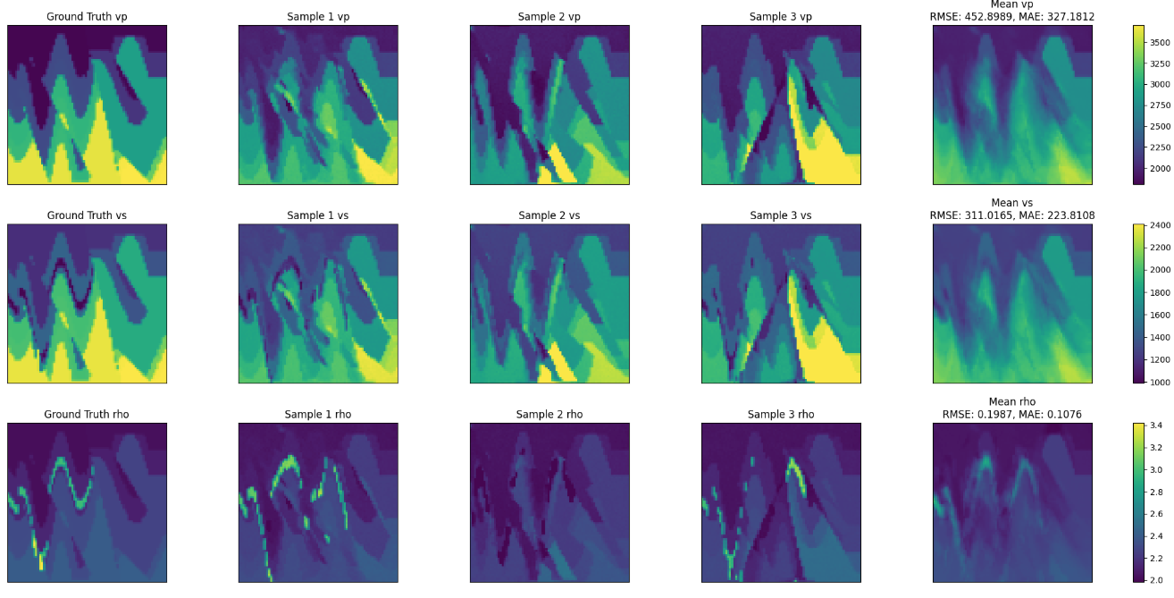
Fig. 55 Zero-shot sampling predictions#
A figure
ensemble_variance.pngcontaining the variance of the ensemble predictions. This indiactes the uncertainty on the predicted subsurface properties, which is useful for example to guide the placement of potential well logs.
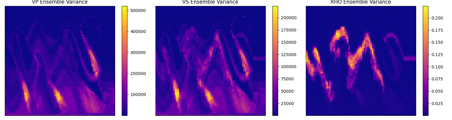
Fig. 56 Zero-shot sampling variance#
A subdirectory
numpycontaining the raw numpy arrays of the predictions, which can be used for further analysis or post-processing.
If Weights & Biases is enabled, the generate.py script also creates a subdirectory specified by ++wandb.results_dir=<path_to_wandb_directory> containing the predictions as Wandb images.
Physics-informed sampling#
The zero-shot sampling procedure is purely data-driven and does not explicitly use any physics information. This shortcoming can be addressed by using physics-informed sampling, following the Diffusion Posterior Sampling (DPS) approach. In this approach, the reverse diffusion SDE is modified to account for a physics-informed guidance term:
In this equation, \(\phi(\mathbf{x}_t, t)\) is the physics-informed guidance term and \(S_c\) is its strength, which can be used to modulate its influence. The guidance term \(\phi(\mathbf{x}_t, t)\) is defined as the likelihood score:
where \(\mathcal{R}\) is the solution operator associated to the wave equation (detailed in the Problem Overview section), \(\hat{\mathbf{x}}_0\) is an estimate of the clean velocity model from the diffusion model, and \(\Sigma\) is a parameter related to the measurement noise. These parameters are defined following an adapted version of the method introduced in Score-based data assimilation (SDA).
Note: The present approach is not true DPS, as the latter is usually based on an unconditional prior score \(\nabla_x \log p(\mathbf{x}_t)\), trained in an unsupervised manner. Instead we use an ad-hoc modification of DPS where we replace the unconditional prior score with a conditional score \(\nabla_x \log p_t(\mathbf{x}_t | \mathbf{y})\), trained in a supervised manner.
The generate.py script implements this sampling procedure by enabling it in the conf/config_generate.yaml file, or by using the following hydra overrides:
python generate.py --config-name=config_generate ++dataset.directory=<path_to_dataset_directory> ++model.checkpoint_path=<path_to_checkpoint> ++generation.sampler.physics_informed=true ++generation.num_ensembles=<size_of_ensemble>
The guidance parameters can be controlled through the ++generation.sampler.physics_informed_guidance field in the configuration.
⚠️ Warning: The default guidance parameters in
conf/config_generate.yamlare only informative and may not be optimal. Finding the optimal guidance parameters typically requires some calibration, which can be achieved by leveraging hydra capabilities for parameter sweep.
Simlarly to the zero-shot sampling procedure, the generate.py script supports ensemble generation, distributed generation through torchrun, Weights & Biases logging, and it still produces outputs in the directory specified by ++io.output_dir=<path_to_output_directory>. For example, the following figure shows a few predictions from the ensemble, as well as the mean prediction and the ground truth velocity model.
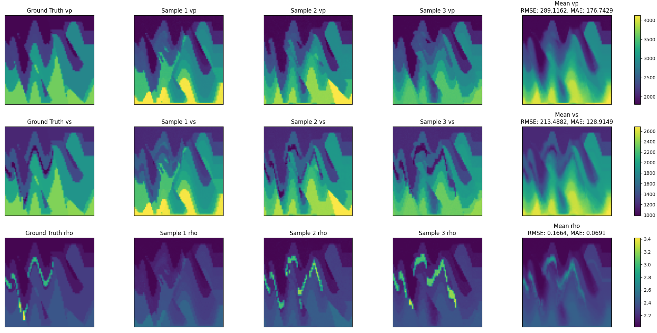
Fig. 57 Physics-informed sampling predictions#
References#
⚠️ Warning: The E-FWI dataset is distributed under a non-commercial license CC BY-NC-SA 4.0.