Domain Parallelism and Shard Tensor#

In scientific AI, one of most challenging aspects in training a model is dealing with extremely high resolution data. In this tutorial, we’ll explore what makes high resolution data so challenging to handle, for both training and inference, and why that’s different from the scaling challenges in other domains (like NLP and image processing). We’ll also take a technical look at how we’re working to streamline high-resolution model training in PhysicsNeMo, and how you can leverage our tools for your own scientific workloads as well.

What Makes Scientific AI Challenging?#

To understand why scientific AI encounters unique challenges in training and inference on high resolution data, let’s take a look at the computational and memory cost of training models and subsequently running inference. “Cost” here refers to two fundamental, high level concepts:

computational cost is how much computing power is needed to complete an operation (and includes a complicated interplay of GPU FLOPs, memory bandwidth, cache sizes, and algorithm efficiencies).
memory costs refer to the amount of GPU memory required to perform the computations.

For all AI models, the memory cost of inference is dominated by just two categories of use:

Model parameters (weights, biases, and encodings) all are required to be loaded into GPU memory for fast access during inference. For a model with N total parameters, each parameter requires four bytes in float32 precision, or two in float16/bfloat16. A rough approximation is that a 100M parameter model requires 400MB of memory in float32 precision. For Large Language Models (LLMs) with billions of parameters, even at inference time, this is a large amount of memory.
Active Data (the inputs and outputs) represent the memory required to actually compute the layers and outputs of the model. For inference, the available memory has to be enough to hold the input data, output data, and model parameters. It must also temporariliy accommodate memory of intermediate activations. As one layer’s output is consumed by the next layer, the total memory needed, typically, never exceeds the requirements of the most memory-intensive layer.

For scientific AI with high resolution data, the memory cost at inference is, typically, dominated by the data.

During training (for a standard training loop), the high resolution of the data is even more challenging. There are two additional memory consumers during model training, in most cases:

Optimizer states (gradients, moments) are needed to accumulate and update the model’s parameters during training. This can be as little memory usage as the model’s parameters for SGD. For more complicated optimizers, like adam, the optimizer must store moments and it must run gradient averages, which increases the usage.
Activations For each layer used during training, PyTorch, typically, saves some component of the layer’s input, output, or other activation as the “intermediate activation” for that layer. In practice, this is a computational optimization to enable the backwards pass to compute and propagate gradients more efficiently. Each layer, however, requires extra memory storage during training that is proportional to the resolution of the input data.

As a cumulative effect, as models continue to stack up layers and save intermediate activations, the activation-related memory required to train a model grows with both the depth of the model and the resolution of the input data. In contrast to LLMs, memory usage for high resolution scientific AI models is dominated by activations, where the models have a modest parameter count.

In PhysicsNeMo, ShardTensor is the domain-parallelism framework. It is used to parallelize the:

high compute
memory costs from the storage of temporary activations

of training and inferencing models on high resolution data.

It is built on top of PyTorch’s DTensor framework. It allows models to divide expensive operations across multiple GPUs.

The remainder of this tutorial will focus on the high level concepts of ShardTensor and domain parallelism. Implementing New Layers for ShardTensor will be covered in a separate tutorial.

Starting with an Example#

Consider a basic 2D convolution operation where the input data to the convolution is spread across two GPUs, and you want to correctly compute the ouput of the convolution, but without ever coalescing the input data on a single GPU.

Applying the convolution to each GPU provides incorrect results. You can simulate this, actually, in PyTorch on one device:

import torch

full_image = torch.randn(1, 8, 1024, 1024)

left_image = full_image[:,:,:512,:]
right_image = full_image[:,:,512:,:]

convolution_operator = torch.nn.Conv2d(8, 8, 3, stride=1, padding=1)

full_output = convolution_operator(full_image)

left_output = convolution_operator(left_image)
right_output = convolution_operator(right_image)

recombined_output = torch.cat([left_output, right_output], dim=2)

# Do the shapes agree?
print(full_output.shape)
print(recombined_output.shape)
# (they should!)

# Do the values agree?
torch.allclose(full_output, recombined_output)
# (they do not!)

To understand why they don’t agree, review the location of the disagreement:

diff = full_output - recombined_output
b_locs, c_locs, h_locs, w_locs = torch.where(torch.abs(diff) > 1e-6)
print(torch.unique(b_locs))
print(torch.unique(c_locs))
print(torch.unique(h_locs))
print(torch.unique(w_locs))

This will produce the following output:

tensor([0])
tensor([0, 1, 2, 3, 4, 5, 6, 7])
tensor([511, 512])
tensor([   0,    1,    2,  ..., 1021, 1022, 1023])

We see in particular that along the height dimension (dim=2), the output is incorrect, but only along the pixels 511 and 512, which is right where the data was split. The problem is that the convolution operator is a local operation, but splitting the data prevents it from seeing the correct neighboring pixels right at the border. You can fix this directly:

# Slice off the data needed on the other image (around the center of the original image)
missing_left_data = right_image[:,:,0:1,:]
missing_right_data = left_image[:,:,-1:,:]

# Add it to the correct image
padded_left_image = torch.cat([left_image, missing_left_data], 2)
padded_right_image = torch.cat([missing_right_data, right_image], 2)

# Recompute convolutions
right_output = convolution_operator(padded_right_image)[:,:,1:,:]
left_output = convolution_operator(padded_left_image)[:,:,:-1,:]
# ^ Need to drop the extra pixels in the output here

recombined_output = torch.cat([left_output, right_output], dim=2)

# Now, the output works correctly:
torch.allclose(recombined_output, full_output)
# True

In the example above, just splitting the data and applying the base operation didn’t give correct results.

In general, for many operations in AI models, splitting the data across GPUs requires extra operations or communication to get everything right.

For gradients to call backward() through this split operation across devices also requires extra operations and communication. But, to get the memory and potential computational benefits of domain parallelism, it’s necessary.

How Does `ShardTensor` Help?#

PyTorch’s DTensor interface already has an interface for a distributed tensor mechanism, and it’s great - great enough, in fact, that ShardTensor is built upon it. However, DTensor is built with a different paradigm of parallelism in mind, including model parallelisms from DeepSpeed and MegaTron - which is supported in pytorch via Fully Sharded Data Parallelism. It has several shortcomings: notably, it can not accommodate data that isn’t distributed uniformly or according to torch.chunk syntax. For scientific data, such as mesh data, point clouds, or anything else irregular, this is a nearly-immediate dead end for deploying domain parallelism. Further, DTensor’s mechanism for implementing parallelism is largely restricted to lower level torch operations - great for broad support in PyTorch, but not as accesible for most developers.

With ShardTensor, we extend the functionality of DTensor in the ways needed to make domain parallelism simpler and easier to apply. In practice, this looks like the following, if you reuse the convolution example from before:

Full Sharded Convolution Example

Listing 1 Example of domain parallel convolution with ShardTensor#

# SPDX-FileCopyrightText: Copyright (c) 2023 - 2024 NVIDIA CORPORATION & AFFILIATES.
# SPDX-FileCopyrightText: All rights reserved.
# SPDX-License-Identifier: Apache-2.0
#
# Licensed under the Apache License, Version 2.0 (the "License");
# you may not use this file except in compliance with the License.
# You may obtain a copy of the License at
#
#     http://www.apache.org/licenses/LICENSE-2.0
#
# Unless required by applicable law or agreed to in writing, software
# distributed under the License is distributed on an "AS IS" BASIS,
# WITHOUT WARRANTIES OR CONDITIONS OF ANY KIND, either express or implied.
# See the License for the specific language governing permissions and
# limitations under the License.

import torch

from torch.distributed.tensor import (
    Shard,
    distribute_module,
)


from physicsnemo.distributed import (
    DistributedManager,
    ShardTensor,
    scatter_tensor,
)

DistributedManager.initialize()
dm = DistributedManager()

###########################
# Single GPU - Create input
###########################
original_tensor = torch.randn(1, 8, 1024, 1024, device=dm.device, requires_grad=True)

###########################################
# Single GPU - Create a single-layer model:
###########################################
conv = torch.nn.Conv2d(8, 8, 3, stride=1, padding=1).to(dm.device)

########################################
# Single GPU - forward + loss + backward
########################################
single_gpu_output = conv(original_tensor)

# This isn't really a loss, just a pretend one that's scalar!
single_gpu_output.mean().backward()
# Copy the gradients produced here - so we don't overwrite them later.
original_tensor_grad = original_tensor.grad.data.clone()

####################
# Single GPU - DONE!
####################


#################
# Sharded - Setup
#################


# DeviceMesh is a pytorch object - you can initialize it directly, or for added
# flexibility physicsnemo can infer up to one mesh dimension for you
# (as a -1, like in a tensor.reshape() call...)
mesh = dm.initialize_mesh(mesh_shape=(-1,), mesh_dim_names=("domain_parallel",))

# A mesh, by the way, refers to devices and not data: it's a mesh of connected
# GPUs in this case, and the python DeviceMesh can be reused as many times as needed.
# That said, it can be decomposed similar to a tensor - multiple mesh axes, and
# you can axis sub-meshes.  Each mesh also has ways to access process groups
# for targeted collectives.


###########################
# Sharded - Distribute Data
###########################

# This is now a tensor across all GPUs, spread on the "height" dimension == 2
# In general, to create a ShardTensor (or DTensor) you need to specify placements.
# Placements must be a list or tuple of `Shard()` or `Replicate()` objects
# from torch.distributed.tensor.
#
# Each index in the tuple represents the placement over the corresponding mesh dimension
# (so, mesh.ndim == len(placements)! )
# `Shard()` takes an argument representing the **tensor** index that is sharded.
# So below, the tensor is sharded over the tensor dimension 2 on the mesh dimension 0.
sharded_tensor = scatter_tensor(
    original_tensor, 0, mesh, (Shard(2),), requires_grad=True
)


################################
# Sharded - distribute the model
################################

# We tell pytorch that the convolution will work on distributed tensors:
# And, over the same mesh!
distributed_conv = distribute_module(conv, mesh)


#####################################
# Sharded - forward + loss + backward
#####################################

# Now, we can do the distributed convolution:
sharded_output = distributed_conv(sharded_tensor)
sharded_output.mean().backward()


############################################
# Sharded - gather up outputs to all devices
############################################

# This triggers a collective allgather.
full_output = sharded_output.full_tensor()
full_grad = sharded_tensor.grad.full_tensor()


#################
# Accuracy Checks
#################

if dm.rank == 0:
    # Only check on rank 0 because we used it's data and weights for the sharded tensor.
    # Check that the output is the same as the single-device output:
    assert torch.allclose(full_output, single_gpu_output, atol=1e-3, rtol=1e-3)
    print(f"Global operation matches local! ")

    # Check that the gradient is correct:
    assert torch.allclose(original_tensor_grad, full_grad)
    print(f"Gradient check passed!")


print(
    f"Distributed grad sharding and local shape: {sharded_tensor.grad._spec.placements}, {sharded_tensor.grad.to_local().shape}"
)

If you run this (torchrun --nproc-per-node 4 conv_example.py), you’ll see the checks on output and gradients both pass. Further, the last line will print:

Distributed grad sharding and local shape: (Shard(dim=2),), torch.Size([1, 8, 256, 1024])

Note that when running this, there was no need to perform manual communication or padding, in either the forward or backward pass. And, though you used a convolution, the details of the operation didn’t need to be explicitly specified. In this case, it just worked.

How does `ShardTensor` work?#

At a high level, DTensor from PyTorch is a concept of a local chunk of a tensor (stored as a torch.Tensor), and a DTensorSpec object which combines a DeviceMesh object representing the group of GPUs the tensor is on, and a description of how that global tensor is distributed (or replicated). ShardTensor extends this API with an addition to the specification to track the shape of each local tensor along sharding axes. This becomes important when the input data is something like a point cloud, rather than an evenly-distributed tensor.

At run time, when an operation in torch has DTensor as input, PyTorch will use a custom dispatcher in DTensor to route and perform operations correctly on the inputs. ShardTensor extends this by intercepting a little higher than DTensor: operations can be intercepted at the functional level, or at the dispatch level, and if ShardTensor has no registered implementation it will fall back to DTensor.

ShardTensor also has dedicated implementations of common reduction operations sum and mean, in order to properly intercept and distribute gradients correctly. This is why, in the example above, you can seamlessly call mean().backward() on a ShardTensor and the gradients will arrive at their proper sharding. No need to do anything special—reducing a ShardTensor will handle this automatically.

There is a substantial amount of care needed to implement layers in ShardTensor (or DTensor!). If you’re interested in doing so for your custom model, please check out a full tutorial on this subject: Implementing New Layers for ShardTensor

When Should You Use `ShardTensor`?#

ShardTensor allows you to train models, even though input data is very high resolution, by bypassing memory limitations without sacrificing accuracy. ShardTensor is a solution enabling you to run training and inference on higher resolution data than a single GPU can accommodate. There are other techniques that might be a better solution for your model and data.

For some use cases, pipeline parallelism can be very powerful. In Pipeline Parallelism the model is divided across two or more devices. Each device contains full layers and activations, but to run the entire model the data is “pipelined”. For example:

input data on GPU 0 is propagated through the local layers
outputs of the last layer on GPU 0 become the inputs to the first layer on GPU 1

Gradients can be computed by running the pipeline in reverse.

Pipeline parallelism enables scaling of GPU memory resources, but does not take much advantage of scaling up GPU compute resources without modifying the training loop.

For example, while GPU 0 is active, all other GPUs are waiting on input. After GPU 0 passes data to GPU 1, GPU 0 sits idle until the backward pass or the next batch of data arrives. For large minibatch data, a good strategy could be to feed each batch of data sequentially, that is, when data passes from GPU 0 to GPU 1, the next batch can start processing on GPU 0.

For inference on large datasets, this is quite efficient, but during training this may cause a computational “bubble” or stall everytime gradients are computed and the model is updated.

Not all models are well supported with pipeline parallelism, for example, a UNet architecture. For these model types, ShardTensor enables you to slice your model by dividing each and every layer over sharded inputs. In terms of model support, this makes more complicated architectures, like UNet, simple because the:

Concatenation of features across the down and up sampling paths is unmodified in the user space.
Sharded implementations become a concat of the local tensor objects.

But, because each layer introduces the additional overhead of communication or coordination, a sharded layer can be less efficient than a purely-local layer. Typically, ShardTensor performs efficiently when the input data is large, and when the ratio of communication time to computation time is small.

For some operations, like sequence-parallel attention using a Ring Mechanism (Ring Attention, the sharded model is:

faster after a certain input data size.
still functional after a massive input size, when a single GPU would run out of memory.

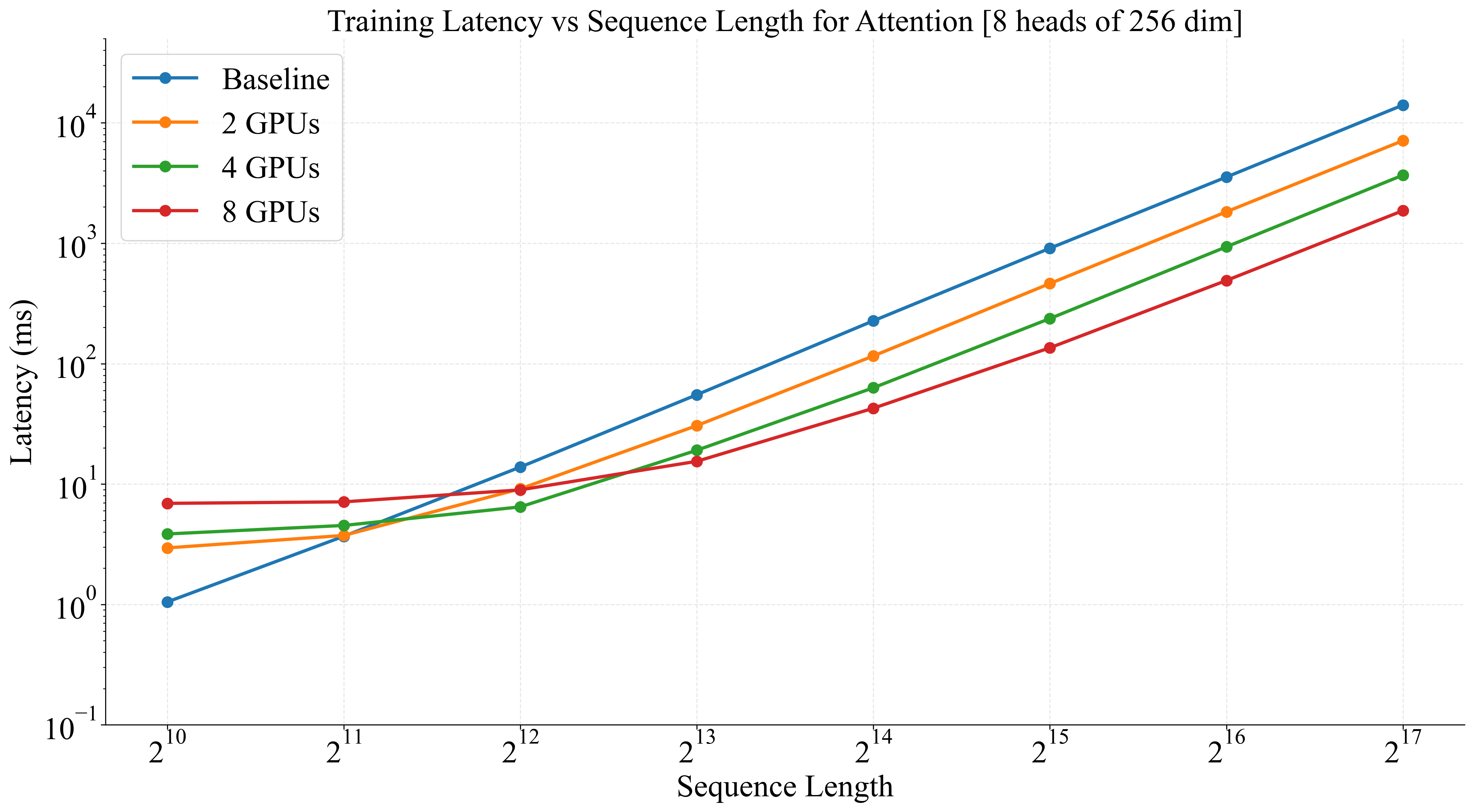
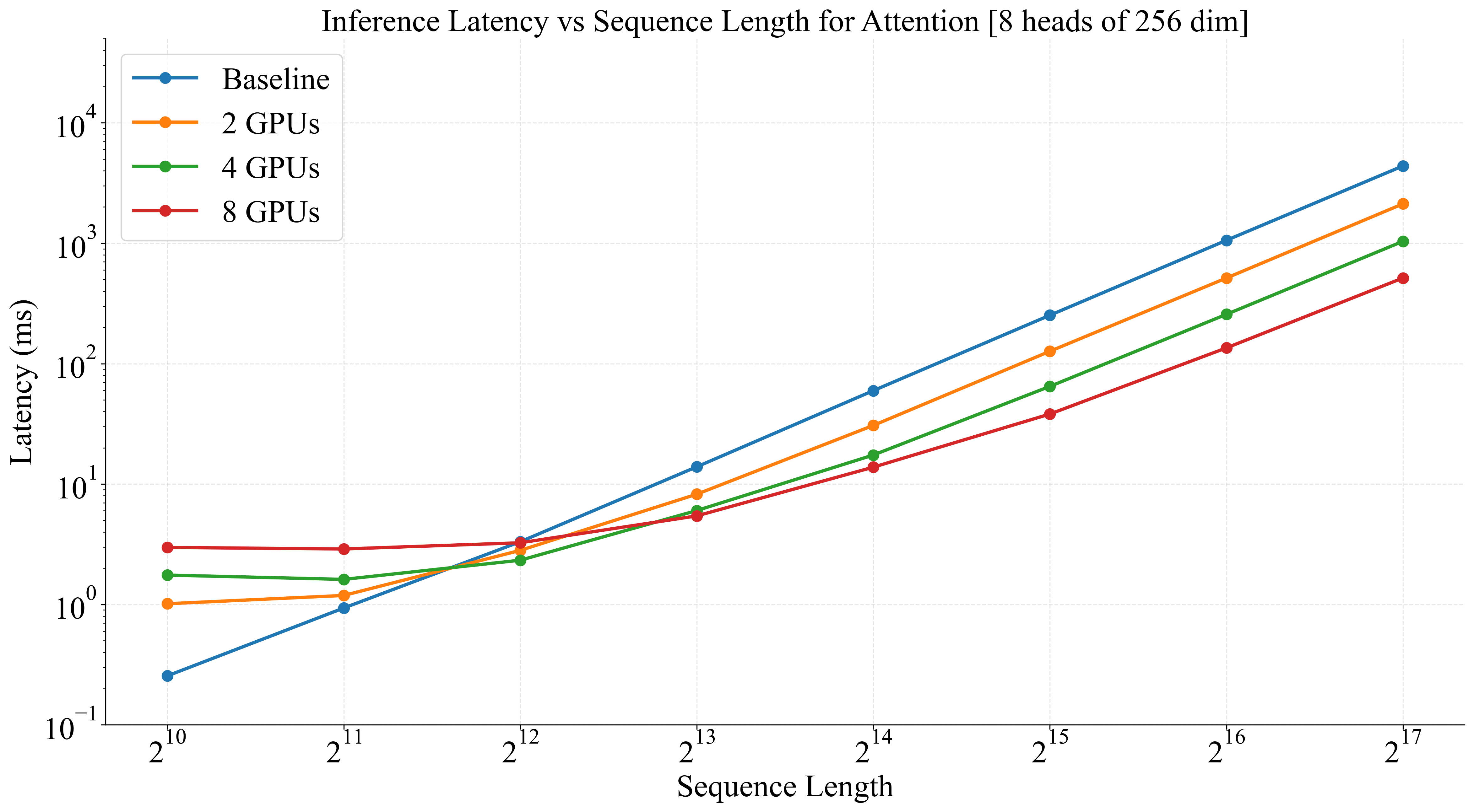
Figure: Left: The latency of a single forward/backward pass, over multiple GPUs with ShardTensor, as compared to a baseline implementation. At larger sequence lengths, scaling efficiency exceeds 95% on 8 GPUs. Right: Inference performance showing how domain parallelism provides reduced latency for high-resolution data processing.

However, a one-layer model isn’t a good representation of actual user code.

Consider the following:

When the GPU kernels are large because the input data is large, ShardTensor scales very efficiently.
When GPU kernels are small, and a model launches many small kernels, ShardTensor will be functional but not as efficient.

In these cases you may have slightly better scaling with pipeline or other parallelism. ShardTensor is still in development and performance optimizations for small kernels are ongoing.

Another technique for dealing with high resolution input data during training is activation checkpointing. In this technique, during the forward pass, activations are moved from GPU memory to CPU memory to make more space available. They are restored during the backward pass when needed, and the rest of the backward pass continues. Compared to pipeline parallelism, this technique can better leverage parallelization across GPUs with standard Data-Parallel scaling. However, it can be limited by GPU/CPU transfer speeds and possible blocking operations. On NVIDIA GPUs with NCCL enabled, the peer-to-peer bandwidth can be significantly higher than CPU-GPU bandwidth (though not all - GraceHopper systems, for example, can efficiently and effectively take advantage of CPU memory offloading). Unlike ShardTensor, the offloading of activations may need tuning and optimization based on GPU system architecture. ShardTensor is designed to work with your model as-is to the greatest possible extent.

In general, if your model meets all of these conditions, consider using ShardTensor for domain parallelism during training:

Your model has relatively large input size even at batch size of 1 - so large, in fact, that you run out of GPU memory trying to train the model with batch size 1.

Note

If your model comfortably fits batch_size=1 training, you will have more efficient training using PyTorch’s DistributedDataParallel.
Your model is composed of supported domain-parallel layers (convolutions, normalizations, upsampling/pooling/reductions, and attention layers).

Note

Not every layer has a domain-parallel implementation in PhysicsNeMo. You can add it to your code yourself if it’s simple (consider a P.R. if you do!) or ask for support on GitHub. How do you know if a layer is supported? Pass a ShardTensor as input to test it.
You have multiple GPUs available (ideally connected with high-performance peer-to-peer path backed by NCCL).

Optimal efficiency when training with ShardTensor is possible if:

Your model is mostly composed of large, compute- or bandwidth-bound kernels rather than very small, latency-bound kernels.
Your model is composed of mostly non-blocking CUDA kernels, allowing the slightly higher overhead of domain parallelism to still fill the GPU queue efficiently.

For inference, ShardTensor can still be useful for lower latency inference on extremely high resolution data. Especially if the model is primarly composed of compute- or bandwidth-bound kernels, and the commmunication overhead is small, ShardTensor can provide reductions of inference latency.

Summary#

In this tutorial, we saw details about PhysicsNeMo’s ShardTensor object, and how it can be used to enable domain parallelism. For more details of how layers are enabled, see Implementing New Layers for ShardTensor. For an example of combining domain parallelism with other parallelisms through FSDP, see fsdp_and_shard_tensor :ref:`Domain Decomposition, ShardTensor and FSDP Tutorial.

Glossary#

DeviceMesh: A PyTorch abstraction that represents a set of connected GPUs. See DeviceMesh. DeviceMesh is particularly useful for multilevel parallelism (data parallel training and domain parallelism, for example).
DTensor: PyTorch’s distributed tensor object. See DTensor.
ShardTensor: PhysicsNeMo’s distributed extension to DTensor. In particular, ShardTensor removes requirements for even data distribution (though it’s still optimal for computational load balancing) and implements domain parallel paths for many operations.
NCCL: NVIDIA’s collective communication library for high speed GPU-GPU communication. See NCCL.
DDP: PyTorch’s distributed data parallel training system. See DDP.
FSDP: PyTorch’s fully sharded data parallel training system. FSDP is an superset of DDP, and to use ShardTensor domain parallelism you must use FSDP, not DDP. See FSDP.
DeepSpeed: A distributed training and inference framework for large language models, built fully sharding weights, gradients, and optimizer states. See DeepSpeed.
MegaTron: Another distributed training and inference framework for large language models, built on sharding weights along the channel dimension with optimized Attention collectives. See MegaTron.