Heat Transfer with High Thermal Conductivity

Introduction

This tutorial discusses strategies that can be employed for handling conjugate heat transfer problems with higher thermal conductivities that represent more realistic materials. The Conjugate Heat Transfer tutorial introduced how you can setup a simple conjugate heat transfer problem in PhysicsNeMo Sym. However, the thermal properties in that example do not represent realistic material properties used to manufacture a heatsink or to cool one. Usually the heatsinks are made of a highly conductive material like Aluminum/Copper, and for air cooled cases, the fluid surrounding the heatsink is air. The conductivities of these materials are orders of magnitude different. This causes sharp gradients at the interface and makes the neural network training very complex. This tutorial shows how such properties and scenarios can be handled via appropriate scaling and architecture choices.

This tutorial presents two scenarios, one where both the materials are solids but the conductivity ratio between the two is \(10^4\) and a second scenario where there is conjugate heat transfer between a solid and a fluid where the solid is copper and fluid is air. The scripts used in this problem can be found in examples/chip_2d/ directory.

2D Solid-Solid Heat Transfer

The geometry of the problem is a simple composite 2D geometry with different material conductivities. The heat source is placed in inside the material of higher conductivity to replicate the actual heatsink and scenario. The objective of this case is to mimic the orders of magnitude difference between Copper \((k=385 \text{ } W/m-K)\) and Air \((k=0.0261 \text{ } W/m-K)\). Therefore, set the conductivity of the heatsink and surrounding solid to 100 and 0.01 respectively.

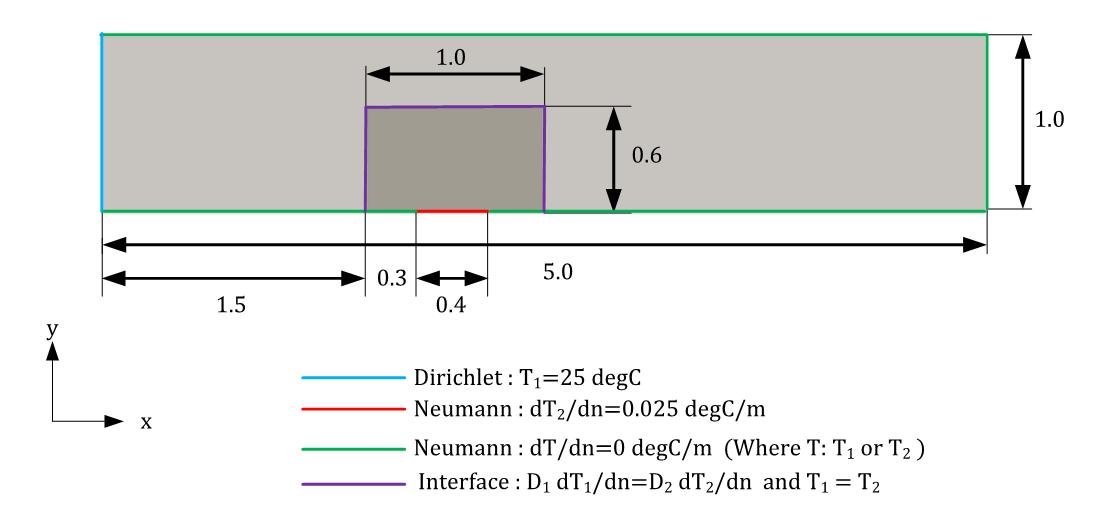
Fig. 182 Geometry for 2D solid-solid case

For this problem, it was observed that using the Modified Fourier Networks with Gaussian frequencies led to the best results. Also, for this problem you can predict the temperatures directly in \((^{\circ} C)\). To achieve this, rescale the network outputs according to the rough range of the target solution, which typically requires some domain knowledge of the problem. It turns out that this simple strategy not only greatly accelerates the training convergence, but also effectively improves the model performance and predictions. The code to setup this problem is shown here:

# SPDX-FileCopyrightText: Copyright (c) 2023 - 2024 NVIDIA CORPORATION & AFFILIATES.
# SPDX-FileCopyrightText: All rights reserved.
# SPDX-License-Identifier: Apache-2.0
#
# Licensed under the Apache License, Version 2.0 (the "License");
# you may not use this file except in compliance with the License.
# You may obtain a copy of the License at
#
#     http://www.apache.org/licenses/LICENSE-2.0
#
# Unless required by applicable law or agreed to in writing, software
# distributed under the License is distributed on an "AS IS" BASIS,
# WITHOUT WARRANTIES OR CONDITIONS OF ANY KIND, either express or implied.
# See the License for the specific language governing permissions and
# limitations under the License.

import os
import warnings

import torch
import numpy as np
from sympy import Symbol, Eq

import physicsnemo.sym
from physicsnemo.sym.hydra import to_absolute_path, PhysicsNeMoConfig
from physicsnemo.sym.utils.io import csv_to_dict
from physicsnemo.sym.solver import Solver
from physicsnemo.sym.domain import Domain
from physicsnemo.sym.geometry.primitives_2d import Rectangle, Line, Channel2D
from physicsnemo.sym.eq.pdes.navier_stokes import GradNormal
from physicsnemo.sym.eq.pdes.diffusion import Diffusion, DiffusionInterface
from physicsnemo.sym.domain.constraint import (
    PointwiseBoundaryConstraint,
    PointwiseInteriorConstraint,
)
from physicsnemo.sym.models.activation import Activation
from physicsnemo.sym.domain.monitor import PointwiseMonitor
from physicsnemo.sym.domain.validator import PointwiseValidator
from physicsnemo.sym.utils.io.plotter import ValidatorPlotter
from physicsnemo.sym.key import Key
from physicsnemo.sym.node import Node
from physicsnemo.sym.models.modified_fourier_net import ModifiedFourierNetArch


@physicsnemo.sym.main(config_path="conf_2d_solid_solid", config_name="config")
def run(cfg: PhysicsNeMoConfig) -> None:
    # add constraints to solver
    # simulation params
    channel_origin = (-2.5, -0.5)
    channel_dim = (5.0, 1.0)
    heat_sink_base_origin = (-1.0, -0.5)
    heat_sink_base_dim = (1.0, 0.2)
    fin_origin = heat_sink_base_origin
    fin_dim = (1.0, 0.6)
    box_origin = (-1.1, -0.5)
    box_dim = (1.2, 1.0)
    source_origin = (-0.7, -0.5)
    source_dim = (0.4, 0.0)

    inlet_temp = 25.0
    conductivity_I = 0.01
    conductivity_II = 100.0
    source_grad = 0.025

    # make list of nodes to unroll graph on
    d_solid_I = Diffusion(T="theta_I", D=1.0, dim=2, time=False)
    d_solid_II = Diffusion(T="theta_II", D=1.0, dim=2, time=False)
    interface = DiffusionInterface(
        "theta_I", "theta_II", conductivity_I, conductivity_II, dim=2, time=False
    )
    gn_solid_I = GradNormal("theta_I", dim=2, time=False)
    gn_solid_II = GradNormal("theta_II", dim=2, time=False)

    solid_I_net = ModifiedFourierNetArch(
        input_keys=[Key("x"), Key("y")],
        output_keys=[Key("theta_I_star")],
        layer_size=128,
        frequencies=("gaussian", 0.2, 64),
        activation_fn=Activation.TANH,
    )
    solid_II_net = ModifiedFourierNetArch(
        input_keys=[Key("x"), Key("y")],
        output_keys=[Key("theta_II_star")],
        layer_size=128,
        frequencies=("gaussian", 0.2, 64),
        activation_fn=Activation.TANH,
    )
    nodes = (
        d_solid_I.make_nodes()
        + d_solid_II.make_nodes()
        + interface.make_nodes()
        + gn_solid_I.make_nodes()
        + gn_solid_II.make_nodes()
        + [
            Node.from_sympy(100 * Symbol("theta_I_star") + 25.0, "theta_I")
        ]  # Normalize the outputs
        + [
            Node.from_sympy(Symbol("theta_II_star") + 200.0, "theta_II")
        ]  # Normalize the outputs
        + [solid_I_net.make_node(name="solid_I_network")]
        + [solid_II_net.make_node(name="solid_II_network")]
    )

    # define sympy variables to parametrize domain curves
    x, y = Symbol("x"), Symbol("y")

    # define geometry
    # channel
    channel = Channel2D(
        channel_origin,
        (channel_origin[0] + channel_dim[0], channel_origin[1] + channel_dim[1]),
    )
    # heat sink
    heat_sink_base = Rectangle(
        heat_sink_base_origin,
        (
            heat_sink_base_origin[0] + heat_sink_base_dim[0],  # base of heat sink
            heat_sink_base_origin[1] + heat_sink_base_dim[1],
        ),
    )
    (fin_origin[0] + fin_dim[0] / 2, fin_origin[1] + fin_dim[1] / 2)
    fin = Rectangle(
        fin_origin, (fin_origin[0] + fin_dim[0], fin_origin[1] + fin_dim[1])
    )
    chip2d = heat_sink_base + fin

    # entire geometry
    geo = channel - chip2d

    # low and high resultion geo away and near the heat sink
    box = Rectangle(
        box_origin,
        (box_origin[0] + box_dim[0], box_origin[1] + box_dim[1]),  # base of heat sink
    )

    lr_geo = geo - box
    hr_geo = geo & box

    (channel_origin[0], channel_origin[0] + channel_dim[0])
    (channel_origin[1], channel_origin[1] + channel_dim[1])

    (box_origin[0], box_origin[0] + box_dim[0])
    (box_origin[1], box_origin[1] + box_dim[1])

    # inlet and outlet
    inlet = Line(
        channel_origin, (channel_origin[0], channel_origin[1] + channel_dim[1]), -1
    )
    outlet = Line(
        (channel_origin[0] + channel_dim[0], channel_origin[1]),
        (channel_origin[0] + channel_dim[0], channel_origin[1] + channel_dim[1]),
        1,
    )

    # make domain
    domain = Domain()

    # inlet
    inlet = PointwiseBoundaryConstraint(
        nodes=nodes,
        geometry=inlet,
        outvar={"theta_I": inlet_temp},
        lambda_weighting={"theta_I": 10.0},
        batch_size=cfg.batch_size.inlet,
    )
    domain.add_constraint(inlet, "inlet")

    # outlet
    outlet = PointwiseBoundaryConstraint(
        nodes=nodes,
        geometry=outlet,
        outvar={"normal_gradient_theta_I": 0},
        batch_size=cfg.batch_size.outlet,
    )
    domain.add_constraint(outlet, "outlet")

    # channel walls insulating
    def walls_criteria(invar, params):
        sdf = chip2d.sdf(invar, params)
        return np.less(sdf["sdf"], -1e-5)

    walls = PointwiseBoundaryConstraint(
        nodes=nodes,
        geometry=channel,
        outvar={"normal_gradient_theta_I": 0},
        batch_size=cfg.batch_size.walls,
        criteria=walls_criteria,
    )
    domain.add_constraint(walls, "channel_walls")

    # solid I interior lr
    interior = PointwiseInteriorConstraint(
        nodes=nodes,
        geometry=lr_geo,
        outvar={"diffusion_theta_I": 0},
        batch_size=cfg.batch_size.interior_lr,
        lambda_weighting={"diffusion_theta_I": 1.0},
    )
    domain.add_constraint(interior, "solid_I_interior_lr")

    # solid I interior hr
    interior = PointwiseInteriorConstraint(
        nodes=nodes,
        geometry=hr_geo,
        outvar={"diffusion_theta_I": 0},
        batch_size=cfg.batch_size.interior_hr,
        lambda_weighting={"diffusion_theta_I": 1.0},
    )
    domain.add_constraint(interior, "solid_I_interior_hr")

    # solid II interior
    interiorS = PointwiseInteriorConstraint(
        nodes=nodes,
        geometry=chip2d,
        outvar={"diffusion_theta_II": 0},
        batch_size=cfg.batch_size.interiorS,
        lambda_weighting={"diffusion_theta_II": 1.0},
    )
    domain.add_constraint(interiorS, "solid_II_interior")

    # solid-solid interface
    def interface_criteria(invar, params):
        sdf = channel.sdf(invar, params)
        return np.greater(sdf["sdf"], 0)

    interface = PointwiseBoundaryConstraint(
        nodes=nodes,
        geometry=chip2d,
        outvar={
            "diffusion_interface_dirichlet_theta_I_theta_II": 0,
            "diffusion_interface_neumann_theta_I_theta_II": 0,
        },
        batch_size=cfg.batch_size.interface,
        lambda_weighting={
            "diffusion_interface_dirichlet_theta_I_theta_II": 10,
            "diffusion_interface_neumann_theta_I_theta_II": 1,
        },
        criteria=interface_criteria,
    )
    domain.add_constraint(interface, name="interface")

    # heat source
    heat_source = PointwiseBoundaryConstraint(
        nodes=nodes,
        geometry=chip2d,
        outvar={"normal_gradient_theta_II": source_grad},
        batch_size=cfg.batch_size.heat_source,
        lambda_weighting={"normal_gradient_theta_II": 1000},
        criteria=(
            Eq(y, source_origin[1])
            & (x >= source_origin[0])
            & (x <= (source_origin[0] + source_dim[0]))
        ),
    )
    domain.add_constraint(heat_source, name="heat_source")

    # chip walls
    chip_walls = PointwiseBoundaryConstraint(
        nodes=nodes,
        geometry=chip2d,
        outvar={"normal_gradient_theta_II": 0},
        batch_size=cfg.batch_size.chip_walls,
        # lambda_weighting={"normal_gradient_theta_II": 1000},
        criteria=(
            Eq(y, source_origin[1])
            & ((x < source_origin[0]) | (x > (source_origin[0] + source_dim[0])))
        ),
    )
    domain.add_constraint(chip_walls, name="chip_walls")

    # add monitor
    monitor = PointwiseMonitor(
        chip2d.sample_boundary(10000, criteria=Eq(y, source_origin[1])),
        output_names=["theta_II"],
        metrics={
            "peak_temp": lambda var: torch.max(var["theta_II"]),
        },
        nodes=nodes,
    )
    domain.add_monitor(monitor)

    # add validation data
    file_path = "openfoam/2d_solid_solid_D1.csv"
    if os.path.exists(to_absolute_path(file_path)):
        mapping = {"Points:0": "x", "Points:1": "y", "Temperature": "theta_I"}
        openfoam_var = csv_to_dict(to_absolute_path(file_path), mapping)
        openfoam_var["x"] += channel_origin[0]  # normalize pos
        openfoam_var["y"] += channel_origin[1]
        openfoam_invar_solid_I_numpy = {
            key: value for key, value in openfoam_var.items() if key in ["x", "y"]
        }
        openfoam_outvar_solid_I_numpy = {
            key: value for key, value in openfoam_var.items() if key in ["theta_I"]
        }
        openfoam_validator_solid_I = PointwiseValidator(
            nodes=nodes,
            invar=openfoam_invar_solid_I_numpy,
            true_outvar=openfoam_outvar_solid_I_numpy,
            plotter=ValidatorPlotter(),
        )
        domain.add_validator(openfoam_validator_solid_I)
    else:
        warnings.warn(
            f"Directory {file_path} does not exist. Will skip adding validators. Please download the additional files from NGC https://catalog.ngc.nvidia.com/orgs/nvidia/teams/physicsnemo/resources/physicsnemo_sym_examples_supplemental_materials"
        )

    file_path = "openfoam/2d_solid_solid_D2.csv"
    if os.path.exists(to_absolute_path(file_path)):
        mapping = {"Points:0": "x", "Points:1": "y", "Temperature": "theta_II"}
        openfoam_var = csv_to_dict(to_absolute_path(file_path), mapping)
        openfoam_var["x"] += channel_origin[0]  # normalize pos
        openfoam_var["y"] += channel_origin[1]
        openfoam_invar_solid_II_numpy = {
            key: value for key, value in openfoam_var.items() if key in ["x", "y"]
        }
        openfoam_outvar_solid_II_numpy = {
            key: value for key, value in openfoam_var.items() if key in ["theta_II"]
        }
        openfoam_validator_solid_II = PointwiseValidator(
            nodes=nodes,
            invar=openfoam_invar_solid_II_numpy,
            true_outvar=openfoam_outvar_solid_II_numpy,
            plotter=ValidatorPlotter(),
        )
        domain.add_validator(openfoam_validator_solid_II)
    else:
        warnings.warn(
            f"Directory {file_path} does not exist. Will skip adding validators. Please download the additional files from NGC https://catalog.ngc.nvidia.com/orgs/nvidia/teams/physicsnemo/resources/physicsnemo_sym_examples_supplemental_materials"
        )

    # make solver
    slv = Solver(cfg, domain)

    # start solver
    slv.solve()


if __name__ == "__main__":
    run()

You can monitor the Tensorboard plots to see the convergence of the simulation. The following table summarizes a comparison of the peak temperature achieved by the heat sink between the Commercial solver and PhysicsNeMo Sym results.

Table 9 Comparison of the peak temperature with the reference values

Property	OpenFOAM (Reference)	PhysicsNeMo Sym (Predicted)
Peak temperature \((^{\circ} C)\)	\(180.24\)	\(180.28\)

This figure visualizes the solution.

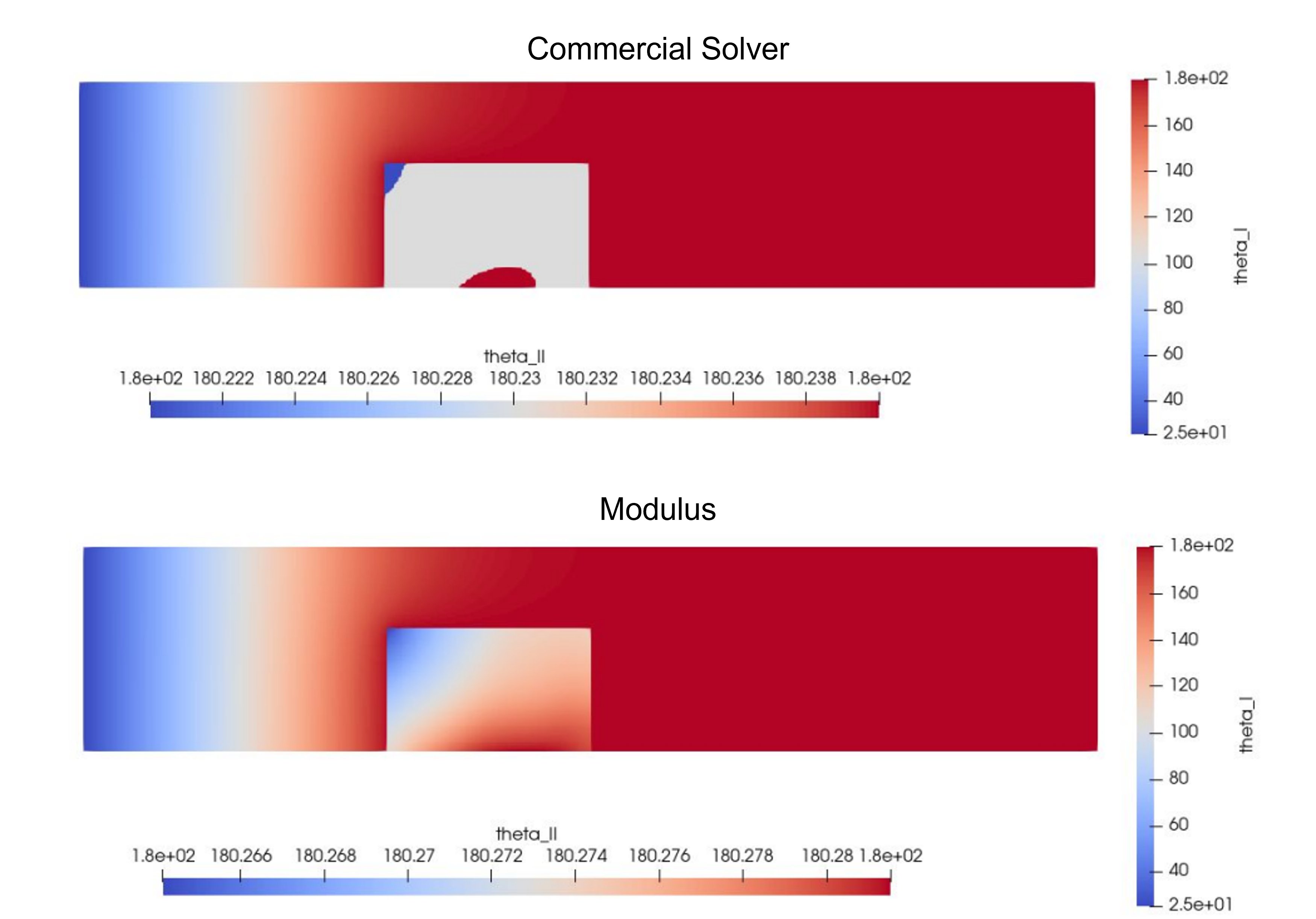
Fig. 183 Results for 2D solid-solid case

2D Solid-Fluid Heat Transfer

The geometry of the problem is very similar to the earlier case, except that now you have a fluid surrounding the solid chip and the dimensions of the geometry are more representative of a real heatsink geometry scales. The real properties for air and copper will also be used in this example. This example is also a good demonstrator for nondimensionalizing the properties/geometries to improve the neural network training. This figure shows the geometry and measurements for this problem.

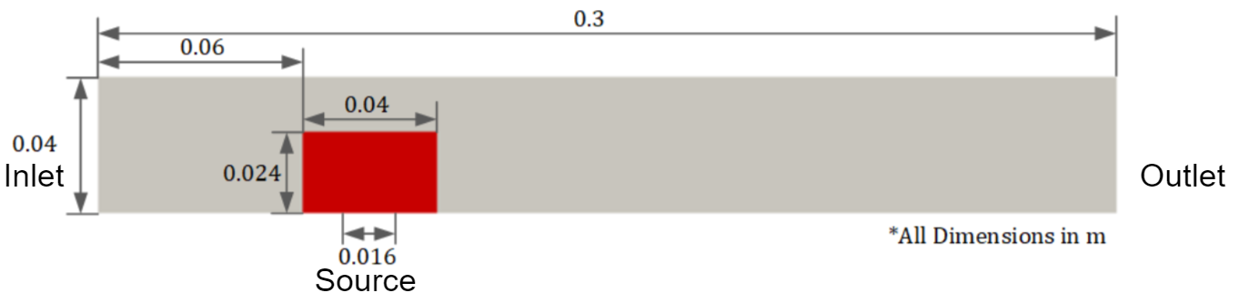
Fig. 184 Geometry for 2D solid-fluid case

For this problem you can employ the same strategies for the heat solution that was used in the solid-solid case and use the Modified Fourier Networks with Gaussian frequencies. The flow solution and heat solution is one way coupled. Use the same multi-phase training approach that was introduced in Conjugate Heat Transfer. A similar approach with rescaling of the network outputs is taken to improve the performance of the model.

The code for solving the flow is very similar to the other examples such as Scalar Transport: 2D Advection Diffusion and Conjugate Heat Transfer. The heat setup is also similar to the solid-solid case that was covered earlier. See examples/chip_2d/chip_2d_solid_fluid_heat_transfer_flow.py and examples/chip_2d/chip_2d_solid_fluid_heat_transfer_heat.py for more details on the definitions of flow/heat constraints and boundary conditions.

The figure below visualizes the thermal solution in solid and fluid. You can observe that PhysicsNeMo Sym prediction does a much better job in predicting the temperature continuity at the interface when compared to the commercial solution. We believe these differences in the solver results are due to the discretization errors and can be potentially fixed by improving the grid resolution at the interface. PhysicsNeMo Sym prediction however does not suffer from such errors and the physical constraints are respected to a better degree of accuracy.

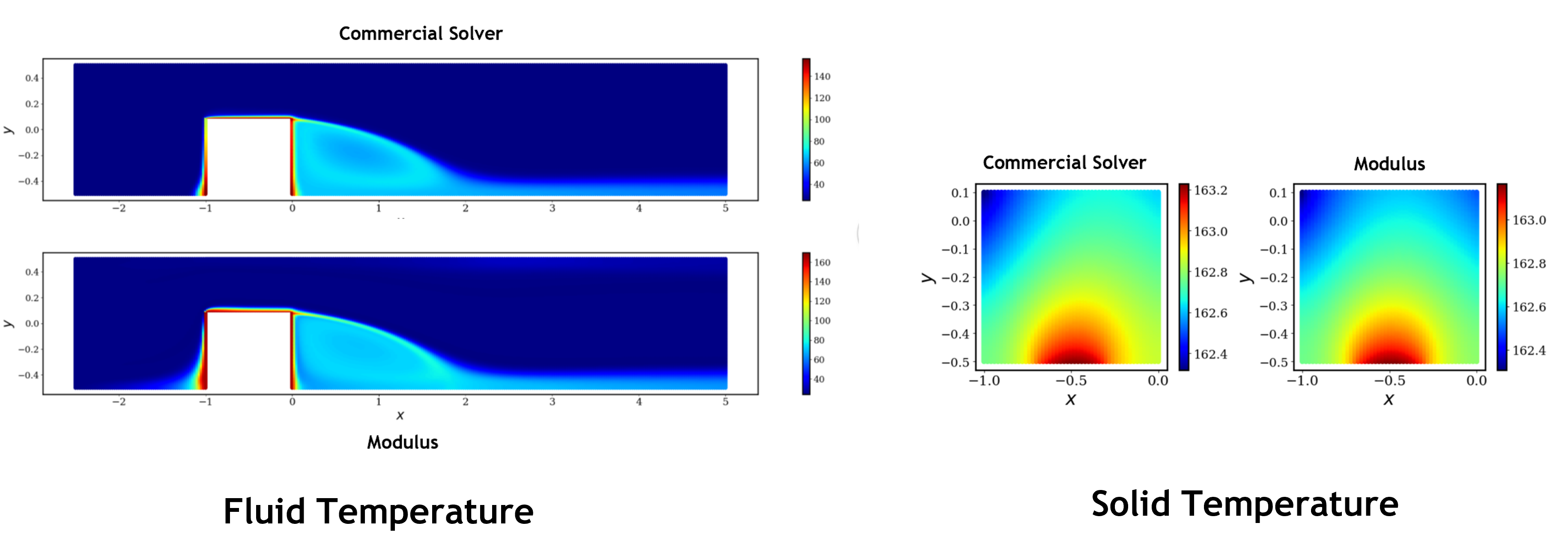
Fig. 185 Results for 2D solid-fluid case