Turbulent physics: Zero Equation Turbulence Model#
Introduction#
This tutorial walks you through the process of adding a algebraic (zero equation) turbulence model to the PhysicsNeMo Sym simulations. In this tutorial you will learn the following:
How to use the Zero equation turbulence model in PhysicsNeMo Sym.
How to create nodes in the graph for arbitrary variables.
Note
This tutorial assumes that you have completed the Introductory Example tutorial on Lid Driven Cavity Flow and have familiarized yourself with the basics of the PhysicsNeMo Sym APIs.
Problem Description#
In this tutorial you will add the zero equation turbulence for a Lid Driven Cavity flow. The problem setup is very similar to the one found in the Introductory Example. The Reynolds number is increased to 1000. The velocity profile is kept the same as before. To increase the Reynolds Number, the viscosity is reduced to 1 × 10⁻⁴ \(m^2/s\).
Case Setup#
The case set up in this tutorial is very similar to the example in Introductory Example. It only describes the additions that are made to the previous code.
Note
The python script for this problem can be found at examples/ldc/ldc_2d_zeroEq.py
Importing the required packages#
Import PhysicsNeMo Sym’ ZeroEquation to help setup the problem.
Other import are very similar to previous LDC.
# limitations under the License.

import os
import warnings

from sympy import Symbol, Eq, Abs
import torch
import physicsnemo.sym
from physicsnemo.sym.hydra import to_absolute_path, instantiate_arch, PhysicsNeMoConfig
from physicsnemo.sym.utils.io import csv_to_dict
from physicsnemo.sym.solver import Solver
from physicsnemo.sym.domain import Domain
from physicsnemo.sym.geometry.primitives_2d import Rectangle

from physicsnemo.sym.domain.constraint import (
    PointwiseBoundaryConstraint,
    PointwiseInteriorConstraint,
)
from physicsnemo.sym.domain.monitor import PointwiseMonitor
from physicsnemo.sym.domain.validator import PointwiseValidator
from physicsnemo.sym.domain.inferencer import PointwiseInferencer
from physicsnemo.sym.eq.pdes.navier_stokes import NavierStokes
from physicsnemo.sym.eq.pdes.turbulence_zero_eq import ZeroEquation
Defining the Equations, Networks and Nodes#
In addition to the Navier-Stokes equation, the Zero Equation turbulence
model is included by instantiating the ZeroEquation equation class.
The kinematic viscosity \(\nu\) in the Navier-Stokes equation is a now a sympy expression
given by the ZeroEquation.
The ZeroEquation turbulence model provides the
effective viscosity \((\nu+\nu_t)\) to the Navier-Stokes equations.
The kinematic viscosity of the fluid calculated based on the Reynolds
number is given as an input to the ZeroEquation class.
The Zero Equation turbulence model is defined in the equations below. Note, \(\mu_t = \rho \nu_t\).
Where, \(l_m\) is the mixing length, \(d\) is the normal distance from wall, \(d_{max}\) is maximum normal distance and \(\sqrt{G}\) is the physicsnemo of mean rate of strain tensor.
The zero equation turbulence model requires normal distance
from no slip walls to compute the turbulent viscosity. For most examples,
signed distance field (SDF) can act as a normal distance. When the geometry is generated
using either the PhysicsNeMo Sym’ geometry module/tesselation module you have access to the sdf
variable similar to the other coordinate variables when used in interior sampling. Since
zero equation also computes the derivatives of the viscosity, when using the PointwiseInteriorConstraint,
you can pass an argument that says compute_sdf_derivatives=True. This will compute
the required derivatives of the SDF like sdf__x, sdf__y, etc.
def run(cfg: PhysicsNeMoConfig) -> None:
    # add constraints to solver
    # make geometry
    height = 0.1
    width = 0.1
    x, y = Symbol("x"), Symbol("y")
    rec = Rectangle((-width / 2, -height / 2), (width / 2, height / 2))

    # make list of nodes to unroll graph on
    ze = ZeroEquation(nu=1e-4, dim=2, time=False, max_distance=height / 2)
    ns = NavierStokes(nu=ze.equations["nu"], rho=1.0, dim=2, time=False)
    flow_net = instantiate_arch(
        input_keys=[Key("x"), Key("y")],
        output_keys=[Key("u"), Key("v"), Key("p")],
        cfg=cfg.arch.fully_connected,
    )

    nodes = (
Setting up domain, adding constraints and running the solver#
This section of the code is very similar to LDC tutorial, so the code and final results is presented here.
    )

    # make ldc domain
    ldc_domain = Domain()

    # top wall
    top_wall = PointwiseBoundaryConstraint(
        nodes=nodes,
        geometry=rec,
        outvar={"u": 1.5, "v": 0},
        batch_size=cfg.batch_size.TopWall,
        lambda_weighting={"u": 1.0 - 20 * Abs(x), "v": 1.0},  # weight edges to be zero
        criteria=Eq(y, height / 2),
    )
    ldc_domain.add_constraint(top_wall, "top_wall")

    # no slip
    no_slip = PointwiseBoundaryConstraint(
        nodes=nodes,
        geometry=rec,
        outvar={"u": 0, "v": 0},
        batch_size=cfg.batch_size.NoSlip,
        criteria=y < height / 2,
    )
    ldc_domain.add_constraint(no_slip, "no_slip")

    # interior
    interior = PointwiseInteriorConstraint(
        nodes=nodes,
        geometry=rec,
        outvar={"continuity": 0, "momentum_x": 0, "momentum_y": 0},
        batch_size=cfg.batch_size.Interior,
        compute_sdf_derivatives=True,
        lambda_weighting={
            "continuity": Symbol("sdf"),
            "momentum_x": Symbol("sdf"),
            "momentum_y": Symbol("sdf"),
        },
    )
    ldc_domain.add_constraint(interior, "interior")

    # add validator
    file_path = "openfoam/cavity_uniformVel_zeroEqn_refined.csv"
    if os.path.exists(to_absolute_path(file_path)):
        mapping = {
            "Points:0": "x",
            "Points:1": "y",
            "U:0": "u",
            "U:1": "v",
            "p": "p",
            "d": "sdf",
            "nuT": "nu",
        }
        openfoam_var = csv_to_dict(to_absolute_path(file_path), mapping)
        openfoam_var["x"] += -width / 2  # center OpenFoam data
        openfoam_var["y"] += -height / 2  # center OpenFoam data
        openfoam_var["nu"] += 1e-4  # effective viscosity
        openfoam_invar_numpy = {
            key: value
            for key, value in openfoam_var.items()
            if key in ["x", "y", "sdf"]
        }
        openfoam_outvar_numpy = {
            key: value for key, value in openfoam_var.items() if key in ["u", "v", "nu"]
        }
        openfoam_validator = PointwiseValidator(
            nodes=nodes,
            invar=openfoam_invar_numpy,
            true_outvar=openfoam_outvar_numpy,
            batch_size=1024,
            plotter=ValidatorPlotter(),
            requires_grad=True,
        )
        ldc_domain.add_validator(openfoam_validator)

        # add inferencer data
        grid_inference = PointwiseInferencer(
            nodes=nodes,
            invar=openfoam_invar_numpy,
            output_names=["u", "v", "p", "nu"],
            batch_size=1024,
            plotter=InferencerPlotter(),
            requires_grad=True,
        )
        ldc_domain.add_inferencer(grid_inference, "inf_data")
    else:
        warnings.warn(
            f"Directory {file_path} does not exist. Will skip adding validators. Please download the additional files from NGC https://catalog.ngc.nvidia.com/orgs/nvidia/teams/physicsnemo/resources/physicsnemo_sym_examples_supplemental_materials"
        )

    # add monitors
    global_monitor = PointwiseMonitor(
        rec.sample_interior(4000),
        output_names=["continuity", "momentum_x", "momentum_y"],
        metrics={
            "mass_imbalance": lambda var: torch.sum(
                var["area"] * torch.abs(var["continuity"])
            ),
            "momentum_imbalance": lambda var: torch.sum(
                var["area"]
                * (torch.abs(var["momentum_x"]) + torch.abs(var["momentum_y"]))
            ),
        },
        nodes=nodes,
        requires_grad=True,
    )
    ldc_domain.add_monitor(global_monitor)

    # make solver
    slv = Solver(cfg, ldc_domain)

    # start solver
    slv.solve()


if __name__ == "__main__":
    run()
The results of the turbulent lid driven cavity flow are shown below.
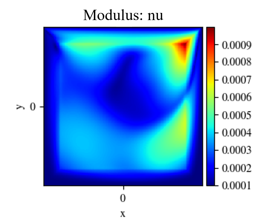
Fig. 116 Visualizing variables from Inference domain#
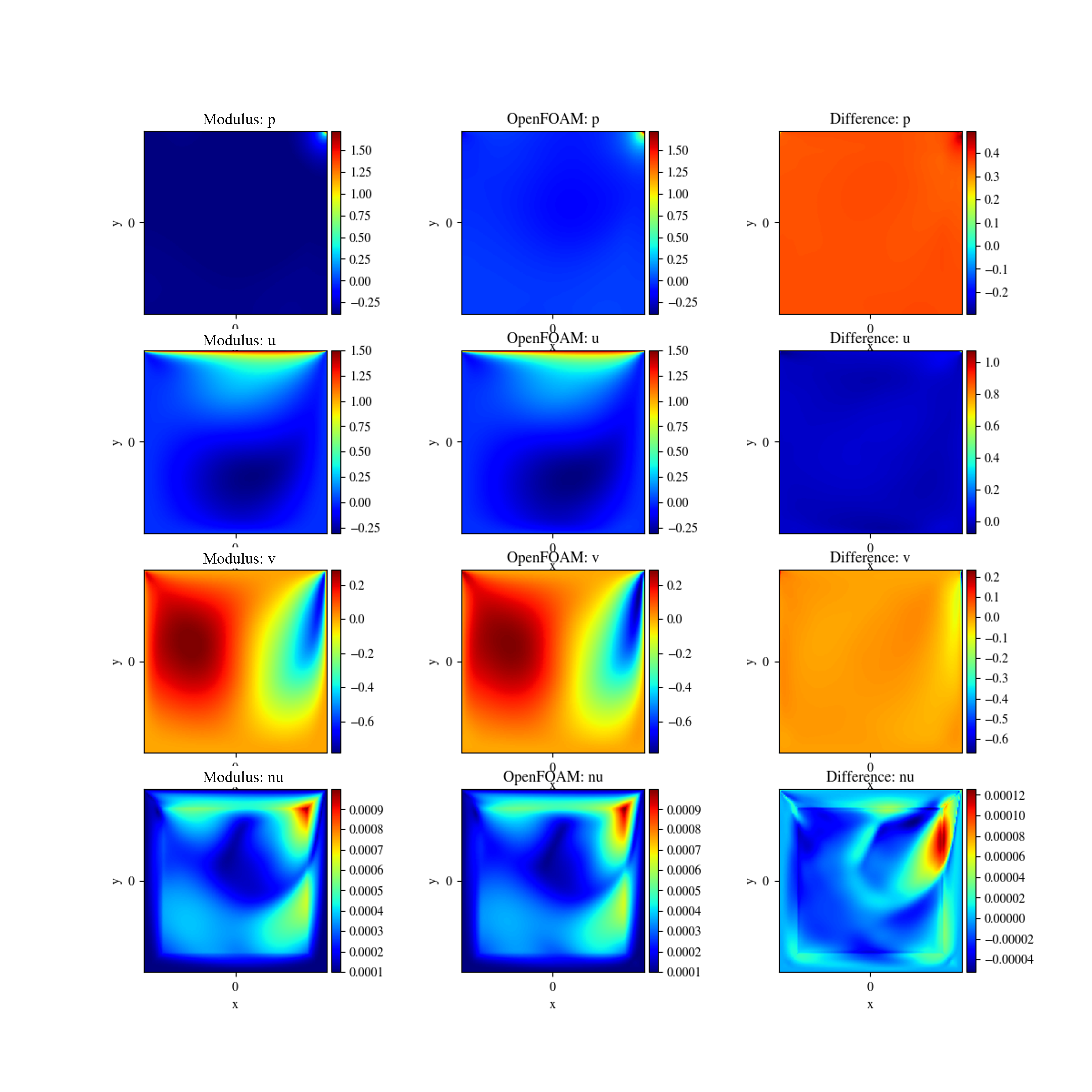
Fig. 117 Comparison with OpenFOAM data. Left: PhysicsNeMo Sym Prediction. Center: OpenFOAM, Right: Difference#