Darcy Flow with Fourier Neural Operator#
Introduction#
In this tutorial, you will use PhysicsNeMo Sym to set up a data-driven model for a 2D Darcy flow using the Fourier Neural Operator (FNO) architecture. You will learn the following:
How to load grid data and set up data-driven constraints
How to create a grid validator node
How to use Fourier Neural Operator architecture in PhysicsNeMo Sym
Note
This tutorial assumes that you are familiar with the basic functionality of PhysicsNeMo Sym and understand the FNO architecture. Please see the Introductory Example and Fourier Neural Operator sections for additional information.
Warning
The Python package gdown is required
for this example if you do not already have the example data downloaded and
converted. Install using pip install gdown.
Problem Description#
Darcy’s law describes the flow rate of a fluid through a porous medium, assuming that the medium is isotropic and a linear relationship between fluid flux and pressure gradient. In the literature, it is often expressed in its 1-dimensional form:
where \(\textbf{q}\) is the fluid flux, \(k\) is the permeability of the medium, \(\mu\) is the dynamic viscosity of the fluid, and \(\nabla p\) is the pressure gradient.
By applying this local 1-dimensional law as the local flux term in a PDE, and combining with the continuity equation, we can generalize this to a PDE in multiple dimensions. This PDE, which we refer to as the “Darcy PDE”, describes the steady-state pressure field of a fluid in a domain, where the fluid is generated throughout the domain at a rate given by a spatially-varying source term. Mathematically, this is a second-order, elliptic PDE:
in which \(u(\textbf{x})\) is the pressure field, \(k(\textbf{x})\) is the permeability field, and \(f(\textbf{x})\) is the source term. Here, we define the domain as a 2D unit square \(D=\left\{x,y \in (0,1)\right\}\) with the boundary condition \(u(\textbf{x})=0, \textbf{x}\in\partial D\). Recall that FNO requires a structured Euclidean input s.t. \(D = \textbf{x}_{i}\) where \(i \in \mathbb{N}_{N\times N}\). Thus both the permeability and flow fields are discretized into a 2D matrix \(\textbf{K}, \textbf{U} \in \mathbb{R}^{N \times N}\). For simplicity of this example, note that we drop the dynamic viscosity term for our PDE without loss of generality.
This problem develops a surrogate model that learns the mapping between a permeability field and the pressure field, \(\textbf{K} \rightarrow \textbf{U}\), for a distribution of permeability fields \(\textbf{K} \sim p(\textbf{K})\). This is a key distinction of this problem from other examples, you are not learning just a single solution but rather a distribution.
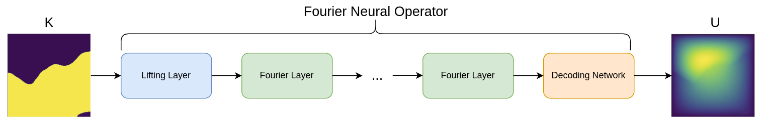
Fig. 129 FNO surrogate model for 2D Darcy flow#
Case Setup#
This example is a data-driven problem. This means that before starting any
coding you need to make sure you have both the training and validation data. The
training and validation datasets for this example can be found on the Fourier
Neural Operator Github page. Here is an automated
script for downloading and converting this dataset. This requires the package
gdown which can easily installed through
pip install gdown.
Note
The python script for this problem can be found at
examples/darcy/darcy_FNO_lazy.py.
Configuration#
The configuration for this problem is fairly standard within PhysicsNeMo Sym.
Note that we have two architectures in the config: one is the pointwise decoder
for FNO and the other is the FNO model which will eventually ingest the decoder.
The most important parameter for FNO models is dimension which tells
PhysicsNeMo Sym to load a 1D, 2D or 3D FNO architecture. nr_fno_layers are
the number of Fourier convolution layers in the model. The size of the latent
features in FNO are determined based on the decoders input key z, in this
case the embedded feature space is 32.
# SPDX-FileCopyrightText: Copyright (c) 2023 - 2024 NVIDIA CORPORATION & AFFILIATES.
# SPDX-FileCopyrightText: All rights reserved.
# SPDX-License-Identifier: Apache-2.0
#
# Licensed under the Apache License, Version 2.0 (the "License");
# you may not use this file except in compliance with the License.
# You may obtain a copy of the License at
#
#     http://www.apache.org/licenses/LICENSE-2.0
#
# Unless required by applicable law or agreed to in writing, software
# distributed under the License is distributed on an "AS IS" BASIS,
# WITHOUT WARRANTIES OR CONDITIONS OF ANY KIND, either express or implied.
# See the License for the specific language governing permissions and
# limitations under the License.

defaults :
  - physicsnemo_default
  - /arch/conv_fully_connected_cfg@arch.decoder
  - /arch/fno_cfg@arch.fno
  - scheduler: tf_exponential_lr
  - optimizer: adam
  - loss: sum
  - _self_

arch:
  decoder:
    input_keys: [z, 32]
    output_keys: sol
    nr_layers: 1
    layer_size: 32

  fno:
    input_keys: coeff
    dimension: 2
    nr_fno_layers: 4
    fno_modes: 12
    padding: 9

scheduler:
  decay_rate: 0.95
  decay_steps: 1000

training:
  rec_results_freq : 1000
  max_steps : 10000

batch_size:
  grid: 32
  validation: 32
Note
PhysicsNeMo Sym configs can allow users to define keys inside the YAML file.
In this instance, input_keys: [z,32] will create a single key of size 32
and input_keys: coeff creates a single input key of size 1.
Loading Data#
For this data-driven problem the first step is to get the training data into
PhysicsNeMo Sym. Prior to loading data, set any normalization value that you
want to apply to the data. For this dataset, calculate the scale and shift
parameters for both the input permeability field and output pressure. Then, set
this normalization inside PhysicsNeMo Sym by providing a shift/scale to each
key, Key(name, scale=(shift, scale)).
    # load training/ test data
    input_keys = [Key("coeff", scale=(7.48360e00, 4.49996e00))]
    output_keys = [Key("sol", scale=(5.74634e-03, 3.88433e-03))]

    download_FNO_dataset("Darcy_241", outdir="datasets/")
    train_path = to_absolute_path(
        "datasets/Darcy_241/piececonst_r241_N1024_smooth1.hdf5"
    )
    test_path = to_absolute_path(
        "datasets/Darcy_241/piececonst_r241_N1024_smooth2.hdf5"
    )
There are two approaches for loading data: First you have eager loading where you immediately read the entire dataset onto memory at one time. Alternatively, you can use lazy loading where the data is loaded on a per example basis as the model needs it for training. The former eliminates potential overhead from reading data from disk during training, however this cannot scale to large datasets. Lazy loading is used in this example for the training dataset to demonstrate this utility for larger problems.
    # make datasets
    train_dataset = HDF5GridDataset(
        train_path, invar_keys=["coeff"], outvar_keys=["sol"], n_examples=1000
    )
    test_dataset = HDF5GridDataset(
        test_path, invar_keys=["coeff"], outvar_keys=["sol"], n_examples=100
    )
This data is in HDF5 format which is ideal for lazy loading using the
HDF5GridDataset object.
Note
The key difference when setting up eager versus lazy loading is the object
passed in the variable dictionaries invar_train and outvar_train. In
eager loading these dictionaries should be of the type Dict[str:
np.array], where each variable is a numpy array of data. Lazy loading uses
dictionaries of the type Dict[str: DataFile], consisting of DataFile
objects which are classes that are used to map between example index and the
datafile.
Initializing the Model#
FNO initialization allows users to define their own pointwise decoder model. Thus we first initialize the small fully-connected decoder network, which we then provide to the FNO model as a parameter.
    # make list of nodes to unroll graph on
    decoder_net = instantiate_arch(
        cfg=cfg.arch.decoder,
        output_keys=output_keys,
    )
    fno = instantiate_arch(
        cfg=cfg.arch.fno,
        input_keys=input_keys,
        decoder_net=decoder_net,
    )
    nodes = [fno.make_node("fno")]
Adding Data Constraints#
For the physics-informed problems in PhysicsNeMo Sym, you typically need to
define a geometry and constraints based on boundary conditions and governing
equations. Here the only constraint is a SupervisedGridConstraint which
performs standard supervised training on grid data. This constraint supports the
use of multiple workers, which are particularly important when using lazy
loading.
    # make domain
    domain = Domain()

    # add constraints to domain
    supervised = SupervisedGridConstraint(
        nodes=nodes,
        dataset=train_dataset,
        batch_size=cfg.batch_size.grid,
        num_workers=4,  # number of parallel data loaders
    )
    domain.add_constraint(supervised, "supervised")
Note
Grid data refers to data that can be defined in a tensor like an image.
Inside PhysicsNeMo Sym this grid of data typically represents a spatial
domain and should follow the standard dimensionality of [batch, channel,
xdim, ydim, zdim] where channel is the dimensionality of your state
variables. Both Fourier and convolutional models use grid-based data to
efficiently learn and predict entire domains in one forward pass, which
contrasts to the pointwise predictions of standard PINN approaches.
Adding Data Validator#
The validation data is then added to the domain using GridValidator which
should be used when dealing with structured data. Recall that unlike the
training constraint, you will use eager loading for the validator. Thus, a
dictionary of numpy arrays are passed to the constraint.
    # add validator
    val = GridValidator(
        nodes,
        dataset=test_dataset,
        batch_size=cfg.batch_size.validation,
        plotter=GridValidatorPlotter(n_examples=5),
    )
    domain.add_validator(val, "test")
Training the Model#
Start the training by executing the python script.
python darcy_FNO_lazy.py
Results and Post-processing#
The checkpoint directory is saved based on the results recording frequency
specified in the rec_results_freq parameter of its derivatives. See
Results Frequency for more information. The network directory folder (in this
case 'outputs/darcy_fno/validators') contains several plots of different
validation predictions. Several are shown below, and you can see that the model
is able to accurately predict the pressure field for permeability fields it had
not seen previously.
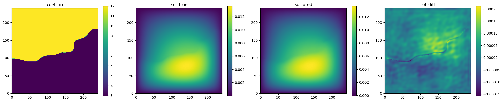
Fig. 130 FNO validation prediction 1. (Left to right) Input permeability, true pressure, predicted pressure, error.#
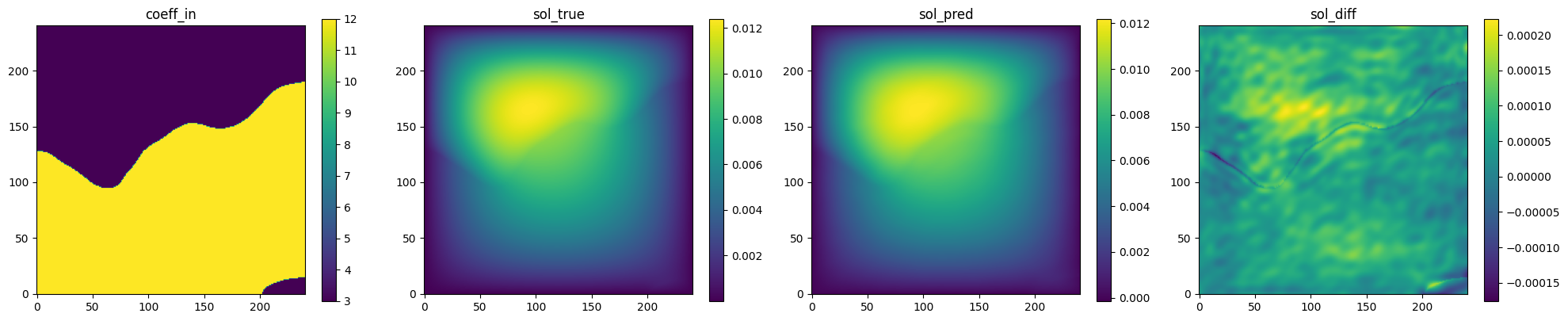
Fig. 131 FNO validation prediction 2. (Left to right) Input permeability, true pressure, predicted pressure, error.#
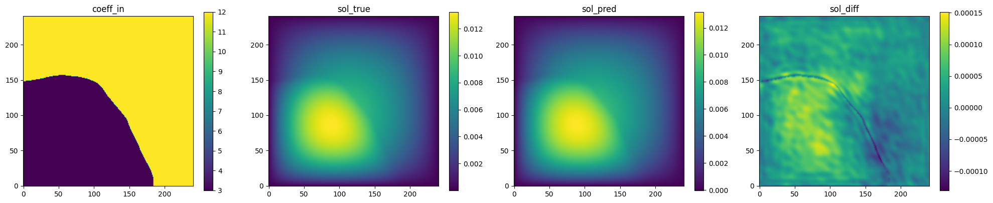
Fig. 132 FNO validation prediction 3. (Left to right) Input permeability, true pressure, predicted pressure, error.#