PhysicsNeMo for PyTorch Users#

PhysicsNeMo is a collection of importable modules for PyTorch developers working on scientific machine learning. You can import the classes and functions that match your task: curator for offline ETL, datapipes for loading training data, mesh for geometry-aware preprocessing, domain parallelism for scaling, Optimized SciML layers and model architectures, symbolic PDE utilities for physics-informed losses.

The useful mental model is:

Use physicsnemo.datapipes when the hard part is getting scientific data from files into GPU-ready tensors.
Use physicsnemo.mesh when the hard part is representing, transforming, differentiating, repairing, or augmenting mesh-like geometry.
Use physicsnemo_curator when the hard part is offline data curation: reading raw engineering/scientific datasets, filtering or transforming them, and writing AI-ready outputs before training begins.
Use physicsnemo.domain_parallel when the hard part is scaling training or large spatial domains.
Use physicsnemo.nn when you want building blocks to use in your own PyTorch modules.
Use physicsnemo.models subpackages when you want to train or evaluate SoTA SciML architecture.
Use physicsnemo.diffusion when you want to experiment with diffusion model training and inference (sampling)
Use physicsnemo.sym when the hard part is adding PDE residuals to a loss.

This page is organized by use case. Each section explains when the module is a good fit, what to import, and how it sits inside a PyTorch workflow.

Quick Module Selection#

If you need to…	Start with…	Typical PyTorch Interefaces
Read HDF5, NumPy, Zarr, VTK, point-cloud, or mesh data	`physicsnemo.datapipes`	`Tensor` or `TensorDict` samples, `Dataloader` -style interface
Curate raw datasets before training	`physicsnemo_curator`	Source, filter, sink ETL pipelines
Process mesh geometry and fields	`physicsnemo.mesh`	`Mesh` or `DomainMesh` objects with tensor fields
Scale a normal PyTorch loop	`physicsnemo.distributed.DistributedManager`	PyTorch `DistributedDataParallel`, FSDP2 (`fully_shard`), and/or `ShardTensor` automatic domain parallelism
Evaluate against SciML SoTA architectures	`physicsnemo.models.transolver` or `physicsnemo.models.dit`	Standard `torch.nn.Module` behavior; `Tensor` input(s) and output(s)
Set up a custom diffusion model	`physicsnemo.diffusion` preconditioners, samplers, noise schedulers and loss functions	Flexible `Tensor`-based protocols
Add symbolic PDE residuals to a loss	`physicsnemo.sym.PDE` and `PhysicsInformer`	Field dictionary in, residual dictionary out

Installation Notes#

The base package is installed as nvidia-physicsnemo and imported as physicsnemo.

Some use cases need optional extras:

pip install nvidia-physicsnemo
pip install "nvidia-physicsnemo[datapipes-extras]"
pip install "nvidia-physicsnemo[mesh-extras]"
pip install "nvidia-physicsnemo[model-extras]"
pip install "nvidia-physicsnemo[sym]"
pip install "nvidia-physicsnemo[gnns]"

Use extras deliberately. For example, physicsnemo.sym depends on symbolic math support, graph neural network examples depend on PyTorch Geometric packages, and some weather or transformer paths may need CUDA-specific packages. Curator is a separate package from the main framework. Install it as physicsnemo-curator and import it as physicsnemo_curator.

Data Loading and Preprocessing with Datapipes#

Use case#

Use physicsnemo.datapipes when your PyTorch model is straightforward but your data is not. Scientific ML data often arrives as HDF5 files, .npz archives, Zarr groups, VTK meshes, point clouds, surface fields, or volume fields. PhysicsNeMo datapipes splits this problem into several customizable abstractions: readers, transforms, datasets, and dataloaders.

Readers load samples from storage and return CPU tensors. Transforms operate on TensorDict objects and can run after device transfer. Dataset combines a reader and transform pipeline, and DataLoader batches samples for a PyTorch loop acting as a drop-in replacement for torch.utils.data.DataLoader.

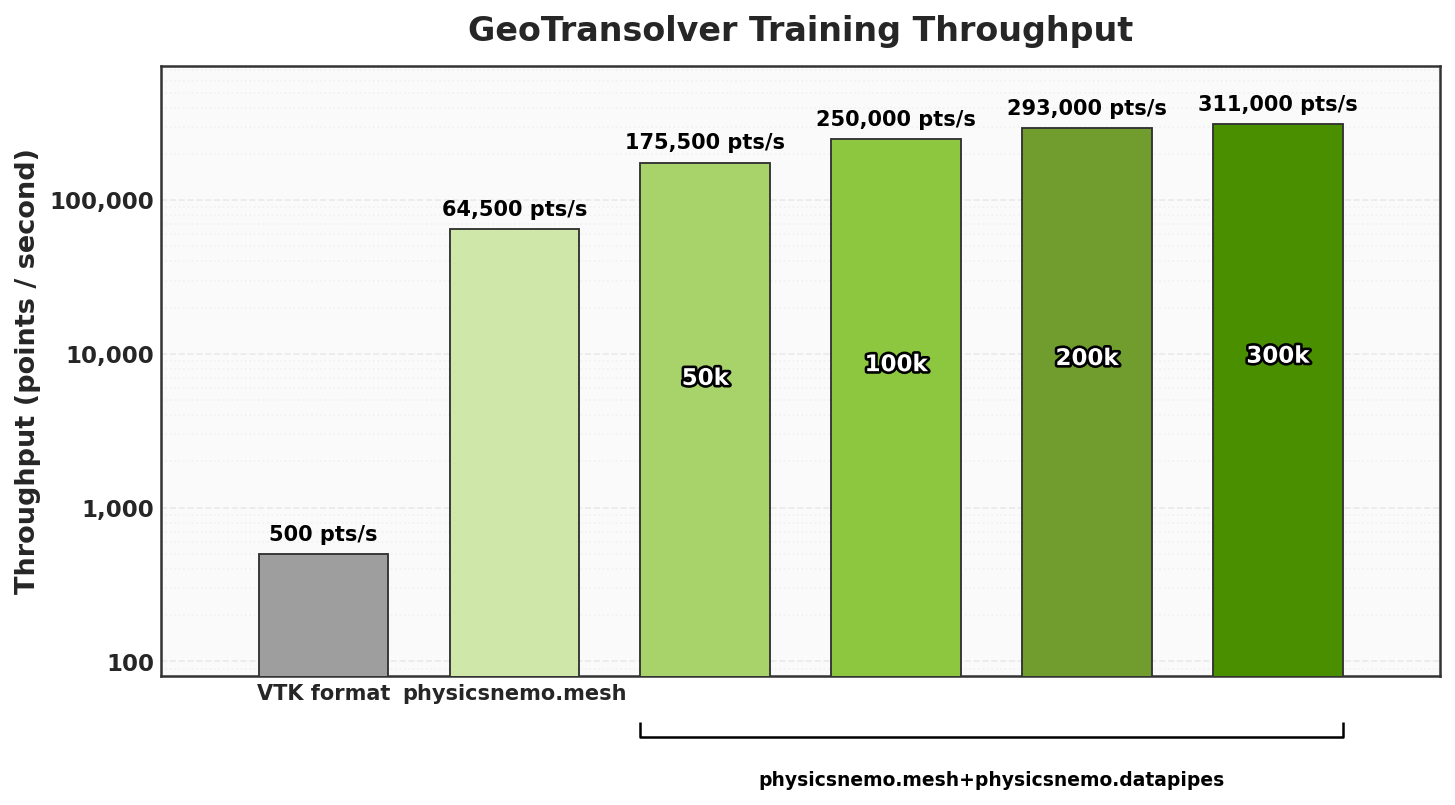
Fig. 14 Performance Throughput of PhysicsNeMo datapipe used for external aerodynamic use cases#

The plot above shows the end-to-end training performance of GeoTransolver, a transformer-based surrogate model for learning over complex CAE geometries and mesh-based simulation data.

The baseline VTK workflow is heavily I/O-bound, achieving only 500 points/second, because each iteration requires expensive serial VTK parsing and full mesh/data reads. Replacing the VTK path with PhysicsNeMo Mesh deserialization increases throughput to 64,500 points/second, showing the significant speed-up of using a CAE-native mesh representation for faster data processing. Read more about PhysicsNemo Mesh [here](Mesh Processing with PhysicsNeMo Mesh).

We further improve throughput by combining PhysicsNeMo Mesh with PhysicsNeMo datapipes and selective reads, so each training iteration loads only the required subset of data instead of reading the full dataset.

What to import#

from physicsnemo.datapipes import Dataset, DataLoader
from physicsnemo.datapipes import HDF5Reader, NumpyReader, ZarrReader
from physicsnemo.datapipes import TensorStoreZarrReader, VTKReader
from physicsnemo.datapipes import Normalize, SubsamplePoints, Compose

Choose a reader based on storage format:

HDF5Reader for HDF5 files or directories of HDF5 samples.
NumpyReader for .npz arrays.
ZarrReader for Zarr groups.
TensorStoreZarrReader for high-performance Zarr reads, especially on large or networked datasets.
VTKReader for .stl, .vtp, or .vtu mesh files.

PyTorch usage#

import torch
from physicsnemo.datapipes import (
    Dataset,
    DataLoader,
    HDF5Reader,
    Normalize,
    SubsamplePoints,
)

device = "cuda" if torch.cuda.is_available() else "cpu"

reader = HDF5Reader(
    "simulation_data.h5",
    fields=["coordinates", "pressure", "velocity"],
    pin_memory=True,
)

transforms = [
    Normalize(
        input_keys=["pressure"],
        method="mean_std",
        means={"pressure": 101325.0},
        stds={"pressure": 5000.0},
    ),
    SubsamplePoints(
        input_keys=["coordinates", "pressure", "velocity"],
        n_points=2048,
    ),
]

dataset = Dataset(reader, transforms=transforms, device=device)
loader = DataLoader(dataset, batch_size=16, shuffle=True)

for batch in loader:
    inputs = torch.cat([batch["coordinates"], batch["velocity"]], dim=-1)
    targets = batch["pressure"]
    predictions = model(inputs)

When point clouds or mesh fields are too large to load completely, use SubsamplePoints to apply the same sampled indices to coordinates and field values. That preserves correspondence between points, pressure, velocity, temperature, normals, or other per-point quantities.

Learn more about PhysicsNeMo datapipes in the documentation here.

Mesh Processing with PhysicsNeMo Mesh#

Use case#

Use physicsnemo.mesh when geometry is part of the learning problem, not just an input array. PhysicsNeMo Mesh represents point clouds, curves, surface meshes, and volume meshes with a common PyTorch-friendly API. Mesh objects can hold point fields, cell fields, and global metadata, move to devices with .to(), and participate in preprocessing pipelines for mesh-based ML.

This is useful for CFD, FEM, CAE, geometry augmentation, boundary-condition handling, mesh repair, spatial queries, differentiating fields on meshes, and extracting features before feeding MeshGraphNet, DoMINO, Transolver, or a custom PyTorch model.

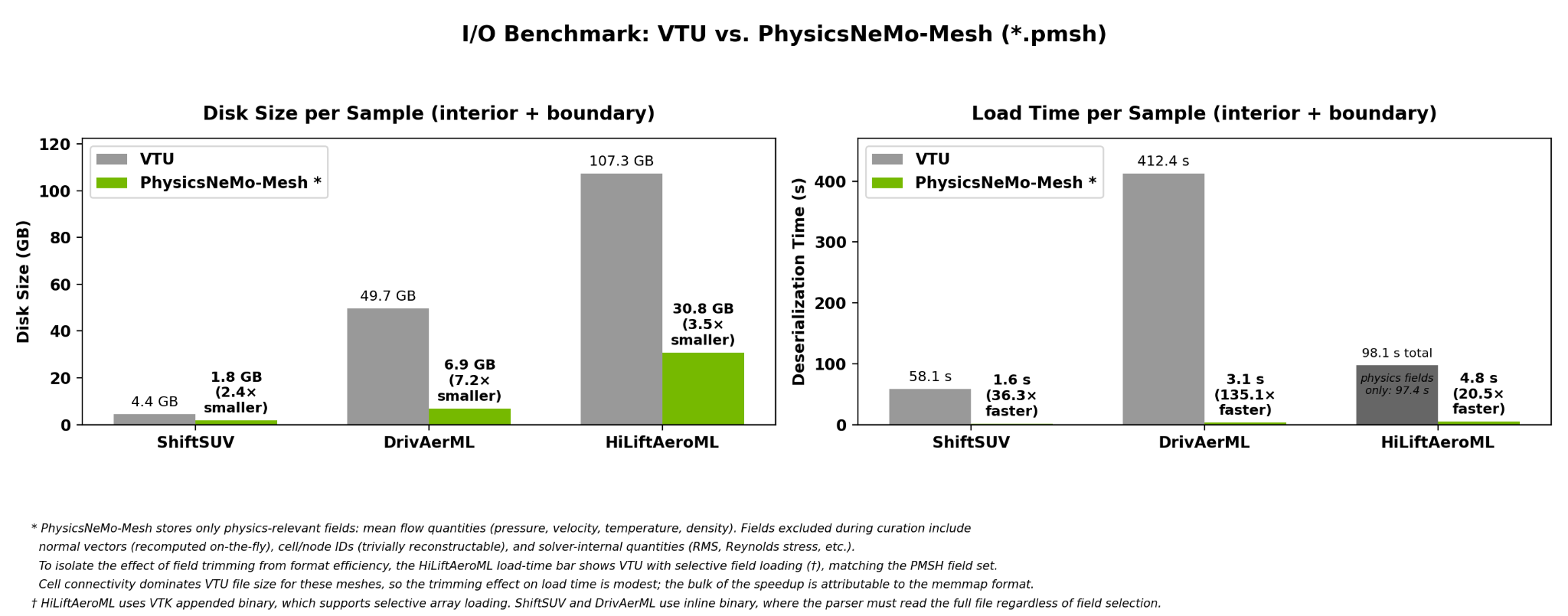
Fig. 15 Graph showing the I/O performance of PhysicsNeMo mesh for ML training#

PhysicsNeMo Mesh stores geometry in a native, memory-mapped format (.pmsh) that loads far faster than solver-native VTU/VTP while preserving the full mesh structure. As the chart shows, PMSH loads are significantly faster than VTU across production datasets, with substantially smaller files on disk. Most of the speedup comes from memory-mapped I/O via TensorDict, which loads tensors byte-for-byte with near-zero parsing overhead, plus trimming fields that are cheap to recompute on the GPU at load time.

What to import#

from physicsnemo.mesh import Mesh, DomainMesh
from physicsnemo.mesh.io import from_pyvista
from physicsnemo.mesh.spatial import BVH
from physicsnemo.mesh.smoothing import smooth_laplacian
from physicsnemo.mesh.remeshing import remesh

Basic mesh usage#

import torch
from physicsnemo.mesh import Mesh

points = torch.tensor([
    [0.0, 0.0],
    [1.0, 0.0],
    [0.5, 1.0],
])
cells = torch.tensor([[0, 1, 2]])

mesh = Mesh(points=points, cells=cells)
mesh.point_data["temperature"] = torch.tensor([300.0, 350.0, 325.0])
mesh.point_data["velocity"] = torch.tensor([
    [1.0, 0.5],
    [0.8, 1.2],
    [0.0, 0.9],
])

mesh = mesh.to("cuda")
mesh.point_data["T"] = mesh.points[:, 0] + 2.0 * mesh.points[:, 1]
mesh = mesh.compute_point_derivatives(keys="T", method="lsq")

Loading geometry from PyVista#

import pyvista as pv
from physicsnemo.mesh.io import from_pyvista

pv_mesh = pv.read("geometry.stl")
mesh = from_pyvista(pv_mesh).to("cuda")

Mesh operations for ML pipelines#

Use Mesh operations to compute features or regularize geometry before training.

from physicsnemo.mesh.spatial import BVH
from physicsnemo.mesh.smoothing import smooth_laplacian
from physicsnemo.mesh.remeshing import remesh

bvh = BVH.from_mesh(mesh)
clean = mesh.clean()
smooth = smooth_laplacian(clean, n_iter=10)
coarse = remesh(smooth, n_clusters=5000)

PhysicsNeMo Mesh also supports subdivision, boundary extraction, adjacency, nearest-cell queries, barycentric interpolation, curvature, normals, geometric transforms, projections, validation, and visualization.

Simulation domains with DomainMesh#

Use DomainMesh when a single mesh is not enough to describe the physics problem. PDE and CFD datasets often have an interior region, named boundary patches, and domain-wide metadata such as Reynolds number, Mach number, angle of attack, reference length, or freestream velocity.

import torch
from physicsnemo.mesh import DomainMesh

domain = DomainMesh(
    interior=interior_mesh,
    boundaries={
        "wall": wall_boundary_mesh,
        "inlet": inlet_boundary_mesh,
        "outlet": outlet_boundary_mesh,
    },
    global_data={
        "reynolds_number": torch.tensor(1.0e6),
        "freestream_velocity": torch.tensor([1.0, 0.0, 0.0]),
    },
)

domain = domain.to("cuda")
domain_aug = domain.rotate(
    angle=0.1,
    transform_point_data=True,
    transform_cell_data=True,
    transform_global_data=True,
)

How it interfaces with PyTorch#

Mesh and DomainMesh are data representations and preprocessing tools. They do not replace neural network models. They help preserve geometry and field semantics long enough to compute features, augment samples, validate meshes, or convert geometry into tensors for a model.

In a PyTorch project, common patterns are:

Curator writes cleaned mesh datasets to disk.
Mesh loads or constructs geometry and computes derived fields.
Datapipes batch the resulting tensors or mesh-derived features.
MeshGraphNet, DoMINO, Transolver, or a custom model consumes the final tensors.

Learn more about PhysicsNeMo Mesh in the documentation here.

Offline Data Curation with PhysicsNeMo Curator#

Use case#

Use PhysicsNeMo Curator when you need an offline ETL pipeline before PyTorch training starts. Datapipes are for feeding batches into a training loop. Curator is for building the dataset those loops will consume: reading raw scientific or engineering files, applying domain-specific filters and transformations, collecting statistics, writing cleaned outputs, and running the pipeline in parallel.

The important naming detail is that Curator is not imported as physicsnemo.curator. It is a separate package installed as physicsnemo-curator and imported as physicsnemo_curator.

What to import#

from physicsnemo_curator import run_pipeline
from physicsnemo_curator.domains.mesh.sources.vtk import VTKSource
from physicsnemo_curator.domains.mesh.filters.mean import MeanFilter
from physicsnemo_curator.domains.mesh.sinks.mesh_writer import MeshSink

Domain extras#

Install the domain extra that matches the data you are curating:

pip install "physicsnemo-curator[mesh]"       # CAE, CFD, VTK meshes
pip install "physicsnemo-curator[da]"         # xarray DataArrays, weather
pip install "physicsnemo-curator[atm]"        # atomic and molecular data
pip install "physicsnemo-curator[dashboard]"  # metrics dashboard

Curator also exposes the psnc command-line tool for interactive pipeline creation and dashboard workflows.

Pipeline usage#

The core pattern is source, filter, sink. A source reads items lazily, filters transform or reject items, and sinks write results.

from physicsnemo_curator import run_pipeline
from physicsnemo_curator.domains.mesh.sources.vtk import VTKSource
from physicsnemo_curator.domains.mesh.filters.mean import MeanFilter
from physicsnemo_curator.domains.mesh.sinks.mesh_writer import MeshSink

pipeline = (
    VTKSource("./cfd_results/")
    .filter(MeanFilter(output="stats.parquet"))
    .write(MeshSink(output_dir="./output/"))
)

# Sequential execution with progress reporting.
results = run_pipeline(pipeline)

# Parallel execution across workers.
results = run_pipeline(pipeline, n_jobs=8, backend="process_pool")

# Some stateful filters need an explicit flush after sequential execution.
pipeline.filters[0].flush()

How it interfaces with PyTorch#

A typical workflow is:

Use Curator to scan raw files, compute dataset statistics, remove invalid samples, normalize schemas, and write curated outputs.
Use physicsnemo.datapipes or a normal PyTorch Dataset to read those curated outputs during training.
Use physicsnemo.models or your own torch.nn.Module for the model.

Use Curator when the dataset itself needs engineering. Use datapipes when the dataset already exists and the training loop needs efficient access.

Learn more about PhysicsNeMo Curator in the documentation here.

Domain Parallelism for Large Spatial Tensors#

Use case#

Use physicsnemo.domain_parallel when normal data parallelism is not enough because individual spatial tensors must be split across ranks. This is a more specialized path for domain decomposition and large-field workloads.

[Include the performance value prop]

What to import#

from torch.distributed.tensor import distribute_module, distribute_tensor, Shard, Replicate
from physicsnemo.domain_parallel import scatter_tensor

Sketch#

# Distribute the model
model = distribute_module(model, device_mesh=domain_mesh, partition_fn=partition_fn)

# Distribute the input tensor
x = scatter_tensor(x, src_rank, domain_mesh, (Shard(input_shard_dimension),))  # shard along input_shard_dimension

# Run the distributed model
out = model(x) # No code changes required inside the model
out_full = out.full_tensor()  # optional: gather sharded output

This is most useful when your input/output tensors are so large you can’t even fit a single sample in memory during training (when normal PyTorch DDP isn’t enough).

Interaction with PyTorch:#

Domain parallelism in physicsnemo is built on ShardTensor, a direct subclass of torch.Tensor that is similar to torch.distributed.tensor.DTensor but with enhanced functionality.

ShardTensor is designed to automatically interface with Tensor and DTensor within PyTorch dispatch, allowing a more seamless user experience and enabling interoperability with pure PyTorch parallelism like FSDP2 (fully_shard).

Learn more about PhysicsNeMo Distributed in the documentation here.

Leverage Optimized SciML Layers#

Use case#

Use physicsnemo.nn when you do not need a full model architecture but do want reusable layers for SciML. The module exports PhysicsNeMo’s Module base class, a direct subclass of torch.nn.Module, and provides a variety of optimized SciML functional operators and layers: fully connected layers, spectral convolutions, embeddings, attention blocks, DiT components, specialized geometry-aware operations, and more.

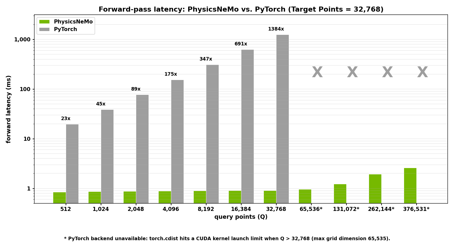
Graph showing the performance of the Ball Query layer in PhysicsNeMo compared to PyTorch — Fig. 16 Graph showing the performance of the Ball Query layer - Custom domain kernels enable scale PyTorch cannot reach. Not just faster, but feasible - Up to 1,384× faster than brute-force PyTorch, with up to 249× less peak memory#

PhysicsNeMo replaces some of the key kernels that dominate CAE training step time; e.g. ball query radius search, scatter/gather interpolation, mesh gradient operators, and signed-distance queries, with implementations that exploit spatial hashing, bounded-volume hierarchies, and structure-aware vectorization. This result in significant speed-up in both end-to-end performance and and per-layer throughput compared to equivalent native PyTorch implementations.

The ball query (radius-based neighbor search), exposed as radius_search, is a clear example. A naive PyTorch implementation computes the full pairwise-distance matrix and then masks it, which is dominated by intermediate-tensor memory traffic and forces you to shrink the point cloud to fit in memory.

What to import#

from physicsnemo.nn import Module, FCLayer
from physicsnemo.nn import SpectralConv1d, SpectralConv2d, SpectralConv3d
from physicsnemo.nn import FourierEmbedding, PositionalEmbedding
from physicsnemo.nn import signed_distance_field, radius_search, legendre_polynomials
from physicsnemo.nn import DiTBlock, ConditioningEmbedder, get_activation

PyTorch usage#

from physicsnemo.nn import Module, FCLayer, SpectralConv2d, get_activation

class MySpectralBlock(Module):
    def __init__(self, channels):
        super().__init__()
        self.spectral = SpectralConv2d(channels, channels, modes1=16, modes2=16)
        self.proj = FCLayer(channels, channels, activation_fn="silu")
        self.act = get_activation("gelu")

    def forward(self, x):
        y = self.spectral(x)
        return self.act(y + x)

Learn more about PhysicsNeMo NN in the documentation here.

SciML Model Zoo#

The physcisnemo.models module offers a wide variety of optimized model architectures that have been developed for and shown to be effective for solving SciML problems. These span more general models to more bespoke/customized architectures, including GNNs, transformers, convolution-based models, neural operators, and hybrid models.

Explore and Evaluate GNNs like MeshGraphNet#

Use MeshGraphNet when your physical system is naturally represented as nodes, edges, and connectivity. Examples include vortex shedding over a mesh, Lagrangian particle or mesh simulations, molecular dynamics graphs, and CAE problems where predictions are attached to mesh nodes.

PhysicsNeMo’s MeshGraphNet works with PyTorch Geometric graph containers. The graph object should represent connectivity. Node and edge features are passed as explicit tensors.

What to import#

from physicsnemo.models.meshgraphnet import MeshGraphNet, BiStrideMeshGraphNet
from torch_geometric.data import Data

PyTorch usage#

import torch
from torch_geometric.data import Data
from physicsnemo.models.meshgraphnet import MeshGraphNet

node_features = batch["node_features"]  # (N_nodes, D_node)
edge_features = batch["edge_features"]  # (N_edges, D_edge)
edge_index = batch["edge_index"]        # (2, N_edges)

graph = Data(edge_index=edge_index, num_nodes=node_features.shape[0])

model = MeshGraphNet(
    input_dim_nodes=node_features.shape[-1],
    input_dim_edges=edge_features.shape[-1],
    output_dim=2,
    processor_size=15,
    aggregation="sum",
).cuda()

pred_node_fields = model(node_features, edge_features, graph)

Do not hide node and edge features inside the PyG graph and expect the model to read them. Pass them explicitly.

Explore and Evaluate Neural operators like DoMINO#

Use DoMINO for aerodynamic surrogate modeling where the model must reason about geometry and predict surface quantities, volume quantities, or both. This is a more specialized interface than FNO or MeshGraphNet. It expects a rich dictionary of geometry, signed distance fields, surface data, volume data, and global parameters.

What to import#

from physicsnemo.models.domino.model import DoMINO
from physicsnemo.models.domino.config import DEFAULT_MODEL_PARAMS

PyTorch usage#

from physicsnemo.models.domino.model import DoMINO
from physicsnemo.models.domino.config import DEFAULT_MODEL_PARAMS

model = DoMINO(
    input_features=3,
    output_features_vol=5,
    output_features_surf=4,
    model_parameters=DEFAULT_MODEL_PARAMS,
).cuda()

data_dict = {
    "geometry_coordinates": batch["geometry_coordinates"],
    "grid": batch["grid"],
    "surf_grid": batch["surf_grid"],
    "sdf_grid": batch["sdf_grid"],
    "sdf_surf_grid": batch["sdf_surf_grid"],
    "surface_mesh_centers": batch["surface_mesh_centers"],
    "surface_normals": batch["surface_normals"],
    "volume_mesh_centers": batch["volume_mesh_centers"],
    "global_params_values": batch["global_params_values"],
    "global_params_reference": batch["global_params_reference"],
}

pred_volume, pred_surface = model(data_dict)

DoMINO is the wrong first choice if you only have a single tensor such as (B, C, H, W). Start with FNO, AFNO, or Transolver for that case.

Explore and Evaluate Transformer based architectures like Transolver#

Use Transolver when you want transformer-style operator learning for PDEs. It supports both structured grids and unstructured point or mesh tokens. This makes it useful when you want one architecture family for regular fields and irregular spatial samples.

What to import#

from physicsnemo.models.transolver import Transolver

Structured grid usage#

from physicsnemo.models.transolver import Transolver

model = Transolver(
    functional_dim=3,
    out_dim=1,
    structured_shape=(64, 64),
    unified_pos=True,
    n_hidden=128,
    n_head=4,
    use_te=False,
).cuda()

fx = batch["state"]  # (B, 64, 64, 3)
pred = model(fx)     # (B, 64, 64, 1)

Unstructured token usage#

model = Transolver(
    functional_dim=2,
    embedding_dim=3,
    out_dim=1,
    structured_shape=None,
    unified_pos=False,
    n_hidden=128,
    n_head=4,
    use_te=False,
).cuda()

fx = batch["features"]      # (B, N, 2)
xyz = batch["coordinates"]  # (B, N, 3)
pred = model(fx, embedding=xyz)

Explore and Evaluate Diffusion based models#

Use the diffusion model backbones when your scientific problem looks like image-to-image correction, generative modeling, super-resolution, downscaling, or denoising on spatial fields. PhysicsNeMo provides UNet-style backbones and a Diffusion Transformer.

What to import#

from physicsnemo.models.diffusion_unets import SongUNet, DhariwalUNet
from physicsnemo.models.diffusion_unets import UNet, CorrDiffRegressionUNet
from physicsnemo.models.diffusion_unets import StormCastUNet
from physicsnemo.models.dit import DiT
from physicsnemo.diffusion import DiffusionModel, Denoiser, Predictor

UNet backbone usage#

import torch
from physicsnemo.models.diffusion_unets import SongUNet

model = SongUNet(
    img_resolution=64,
    in_channels=6,
    out_channels=6,
    label_dim=0,
    augment_dim=0,
    model_channels=64,
    channel_mult=[1, 2, 3],
    num_blocks=4,
    attn_resolutions=[32, 16],
).cuda()

x_noisy = torch.randn(4, 6, 64, 64, device="cuda")
noise_labels = torch.randn(4, device="cuda")
pred = model(x_noisy, noise_labels, None)

DiT backbone usage#

import torch
from physicsnemo.models.dit import DiT

model = DiT(
    input_size=(32, 64),
    patch_size=4,
    in_channels=3,
    out_channels=3,
    condition_dim=8,
).cuda()

x = torch.randn(2, 3, 32, 64, device="cuda")
t = torch.randint(0, 1000, (2,), device="cuda")
condition = torch.randn(2, 8, device="cuda")
out = model(x, t, condition)

The UNet classes are backbones. If you are using PhysicsNeMo preconditioners, losses, or samplers, wrap the backbone with an adapter that matches the diffusion protocol expected by that training stack.

Learn more about PhysicsNeMo Model Zoo in the documentation here.

Incorporate Physics-Informed Losses in your PyTorch training loop#

Use case#

Use physicsnemo.sym when your PyTorch model predicts fields and you want to add a physics residual loss. You define a PDE symbolically with SymPy, then PhysicsInformer computes residual tensors using a selected derivative method.

This is useful for hybrid data-plus-physics training, and inverse problems where physics should constrain the learned fields.

What to import#

from physicsnemo.sym import PDE, PhysicsInformer

The canonical paths are also available:

from physicsnemo.sym.eq.pde import PDE
from physicsnemo.sym.eq.phy_informer import PhysicsInformer

PyTorch usage#

import torch
from sympy import Symbol, Function
from physicsnemo.sym import PDE, PhysicsInformer

class Diffusion(PDE):
    def __init__(self, diffusivity=0.01):
        self.dim = 2
        x, y = Symbol("x"), Symbol("y")
        u = Function("u")(x, y)
        self.equations = {
            "diffusion": -diffusivity * (u.diff(x, 2) + u.diff(y, 2)),
        }

physics = PhysicsInformer(
    required_outputs=["diffusion"],
    equations=Diffusion(),
    grad_method="finite_difference",
    fd_dx=0.01,
    device="cuda",
)

for batch in loader:
    u_pred = model(batch["features"])
    data_loss = torch.nn.functional.mse_loss(u_pred, batch["u_target"])

    residuals = physics.forward({
        "u": u_pred,
        "coordinates": batch["coordinates"],
    })
    physics_loss = (residuals["diffusion"] ** 2).mean()

    loss = data_loss + 0.1 * physics_loss
    loss.backward()

Choose the derivative method based on your data:

autodiff for differentiable coordinate inputs.
finite_difference for regular grids with known spacing.
meshless_finite_difference for point sets.
spectral for suitable regular spectral derivatives.
least_squares for graph or connectivity-based estimates.

Learn more about PhysicsNeMo Sym in the documentation here.

PhysicsNeMo for PyTorch Users#

Quick Module Selection#

Installation Notes#

Data Loading and Preprocessing with Datapipes#

Use case#

What to import#

PyTorch usage#

Mesh Processing with PhysicsNeMo Mesh#

Use case#

What to import#

Basic mesh usage#

Loading geometry from PyVista#

Mesh operations for ML pipelines#

Simulation domains with DomainMesh#

How it interfaces with PyTorch#

Offline Data Curation with PhysicsNeMo Curator#

Use case#

What to import#

Domain extras#

Pipeline usage#

How it interfaces with PyTorch#

Domain Parallelism for Large Spatial Tensors#

Use case#

What to import#

Sketch#

Interaction with PyTorch:#

Leverage Optimized SciML Layers#

Use case#

What to import#

PyTorch usage#

SciML Model Zoo#

Explore and Evaluate GNNs like MeshGraphNet#

What to import#

PyTorch usage#

Explore and Evaluate Neural operators like DoMINO#

What to import#

PyTorch usage#

Explore and Evaluate Transformer based architectures like Transolver#

What to import#

Structured grid usage#

Unstructured token usage#

Explore and Evaluate Diffusion based models#

What to import#

UNet backbone usage#

DiT backbone usage#

Incorporate Physics-Informed Losses in your PyTorch training loop#

Use case#

What to import#

PyTorch usage#

References#