Simulation Domains with DomainMesh#
A Mesh represents a single triangulation, such as the interior field of a PDE simulation along with its solution fields. While this is enough to fully specify the solution to a PDE, a well-posed PDE problem formulation requires more information than this. Specifically, a full PDE problem formulation requires:
An interior region, defining the domain on which the PDE is solved
Boundary patches, along with the boundary conditions applied there and any associated values. Collectively, these should form a watertight boundary around the interior region.
In some cases, problem-level metadata, such as parameters of the governing equations (e.g., Reynolds number) or values associated with infinite far-field boundary conditions (e.g., a freestream velocity vector)
The DomainMesh tensorclass groups all of this into a
single object that can be moved between devices, transformed, validated, and
serialized as a unit.
Why DomainMesh?#
The fundamental reason interior and boundary data are hard to represent together is that they are heterogeneous. For example, in fluid dynamics applications, a quantity like “wall shear stress” is only tracked on the boundary of the domain, while a field like “velocity” might only be tracked on the interior mesh (if boundaries are no-slip walls). Likewise, a thermal simulation where one boundary is a Dirichlet temperature boundary condition and another is a Neumann heat flux boundary condition will have semantically-distinct associated fields. If a downstream model is to encode these differently, the data representation cannot collapse them into a single homogeneous structure. Typical ways in which the schema differs between interior and boundary meshes include:
Different manifold dimensions. The interior is typically
Mesh[n, n](a volume or a 2D area). Each boundary patch isMesh[n-1, n]- a surface around a volume, or a curve around an area. You cannot stack interior and boundary cells into the same array because they are not the same shape.Different field schemas across regions. Interior and each boundary type carry their own field sets, determined by the physics of that region. A flat dictionary keyed on field name cannot express this without null-padding for fields that don’t apply everywhere.
Domain-level metadata. Reynolds number, Mach number, angle of attack, and reference length apply to the entire problem and do not naturally live on any specific boundary patch.
When this heterogeneity is collapsed into a flat representation, boundary-condition information is typically lost. The model must then implicitly learn boundary behavior rather than take it as an explicit input, which limits generalization across geometries, flow regimes, and boundary types.
DomainMesh carries each region as its own Mesh with its own
point_data, cell_data, and global_data, grouped under a single
tensorclass that you can move, transform, and serialize as a unit. If you are
familiar with VTK, DomainMesh serves a similar role to a VTK MultiBlock
dataset (.vtm), grouping related meshes under a single structure - but with
the addition of typed boundary semantics and domain-level global metadata. It is
syntactic sugar plus standardization: no new physics, just a standard way to
represent a simulation domain. The design is model-agnostic: prescriptive in
how you represent a simulation domain, not in how models consume it.
Three fields#
A DomainMesh is a tensorclass with three fields. The formal type
signature, with the codimension constraint between interior and
boundaries, is:
from tensordict import tensorclass, TensorDict
from physicsnemo.mesh import Mesh

@tensorclass
class DomainMesh:
    interior: Mesh["n_manifold_dims", "n_spatial_dims"]
    boundaries: TensorDict[str, Mesh["n_manifold_dims - 1", "n_spatial_dims"]]
    global_data: TensorDict
The three fields are:
``interior``: a single
Meshfor the domain interior (a volume mesh for 3D problems, an area mesh for 2D problems, or a point cloud for query-point-only workflows).``boundaries``: a
TensorDictmapping string keys (typically BC type names like"no_slip","freestream","inlet") toMeshobjects representing each boundary patch.``global_data``: a
TensorDictof domain-wide scalars and tensors (Reynolds number, free-stream velocity vector, angle of attack).
Construction enforces that all boundaries share the interior’s
n_spatial_dims (a ValueError is raised if any boundary has a
different spatial dimension). The codimension relationship (each boundary
one manifold dimension lower than the interior) is a convention, not an
enforced invariant. Watertightness (the boundary patches tiling into a
closed surface around the interior) is also not enforced; verify with
dm.is_boundary_watertight() if your data is supposed to satisfy it.
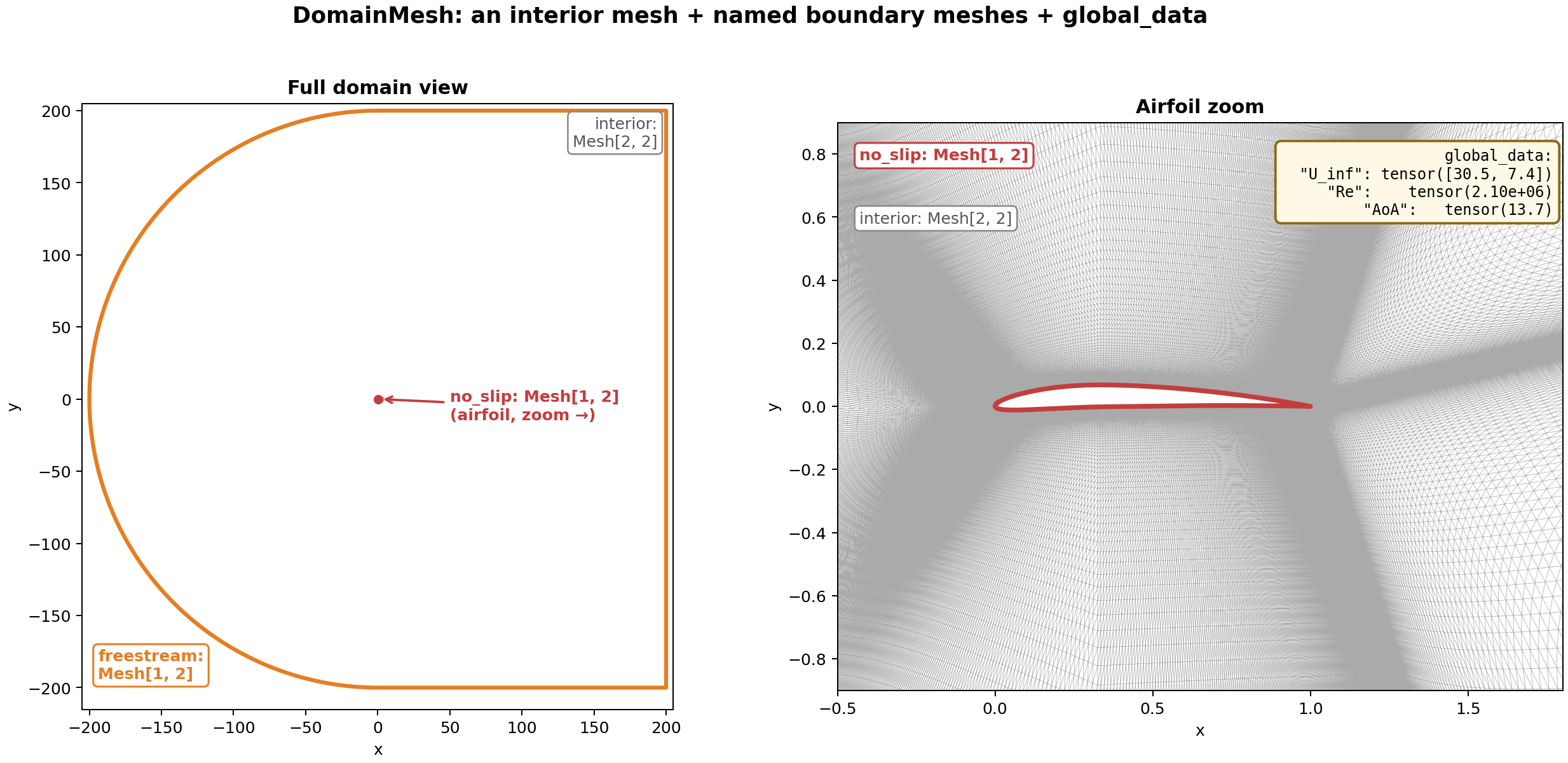
Fig. 18 A DomainMesh for a 2D airfoil simulation. Left: the full domain,
showing the freestream rectangle (orange) as the outer boundary and
the airfoil location at the center. Right: a zoom on the airfoil,
showing the no_slip boundary curve (red) over the interior
triangulation (grey).#
Operations#
Every operation on DomainMesh dispatches through apply(fn), which
calls fn on the interior and on each boundary mesh:
### Apply any Mesh -> Mesh function to all meshes in the domain
dm_subdivided = dm.apply(lambda m: m.subdivide(levels=1, filter="loop"))
dm_cleaned = dm.apply(lambda m: m.clean())
All built-in transforms are thin wrappers around apply:
import numpy as np

### Geometric transforms applied to the entire domain
dm_translated = dm.translate([1.0, 0.0])
dm_rotated = dm.rotate(angle=np.pi / 6)
dm_scaled = dm.scale(2.0)

### Domain-wide repair, subdivision, etc.
dm_clean = dm.clean()
dm_fine = dm.subdivide(levels=1, filter="loop")
The transform methods accept the same transform_*_data flags as
Mesh.rotate (see Using Mesh), so you can co-rotate
vector and tensor fields alongside the geometry.
dm.validate() aggregates per-mesh quality checks across the entire
domain. dm.draw() renders the interior (optionally colored by a scalar
field) and overlays each boundary mesh on top.
Serialization#
DomainMesh.save() writes the whole domain to a *.pdmsh directory
of memory-mapped tensor files, one per leaf tensor. Like *.pmsh for
Mesh, this is a directory - not a single file - with subfolders that
mirror the domain structure (interior, each boundary, global data):
dm.save("/path/to/domain.pdmsh")
dm = DomainMesh.load("/path/to/domain.pdmsh", device="cuda")
Because the on-disk layout is one file per leaf tensor, you can do surgery on individual components without reloading the whole thing: swap a single field, drop a boundary, rename a BC type by editing the directory directly. This matters in practice for large-scale dataset curation, where re-serializing tens of terabytes of mesh data just to add a derived field or fix a bug in one field is prohibitively expensive.
Example: AirFRANS domain#
AirFRANS provides 2D RANS simulations of flow around airfoils. Each sample has three VTK files:
File |
Contents |
|---|---|
|
Triangulated flow field with pressure, velocity, turbulence quantities |
|
Airfoil surface polyline (the no-slip boundary) |
|
Outer-domain polyline (the far-field boundary) |
from pathlib import Path

import pyvista as pv
import torch

from physicsnemo.mesh import DomainMesh, Mesh
from physicsnemo.mesh.io import from_pyvista
from physicsnemo.mesh.projections import project

sample_dir = Path("path/to/airFoil2D_SST_31.468_13.713_3.339_3.51_6.993")
prefix = sample_dir.name

### Interior: drop the constant z-coordinate to project from 3D to 2D
raw_interior = project(
    from_pyvista(pv.read(str(sample_dir / f"{prefix}_internal.vtu"))),
    keep_dims=[0, 1],
    transform_point_data=True,         # also project velocity vectors
)
interior = Mesh(
    points=raw_interior.points,
    cells=raw_interior.cells,
    point_data=raw_interior.point_data.select("p", "U", "nut"),
)

### Boundaries: load and project to 2D
raw_airfoil = project(
    from_pyvista(pv.read(str(sample_dir / f"{prefix}_aerofoil.vtp")), manifold_dim=1),
    keep_dims=[0, 1],
    transform_point_data=True,
)
airfoil = Mesh(
    points=raw_airfoil.points,
    cells=raw_airfoil.cells,
    point_data=raw_airfoil.point_data,
    cell_data=raw_airfoil.cell_data,
)
raw_freestream = project(
    from_pyvista(pv.read(str(sample_dir / f"{prefix}_freestream.vtp")), manifold_dim=1),
    keep_dims=[0, 1],
    transform_point_data=True,
    transform_cell_data=True,
)
freestream = Mesh(
    points=raw_freestream.points,
    cells=raw_freestream.cells,
    point_data=raw_freestream.point_data,
    cell_data=raw_freestream.cell_data,
)

dm = DomainMesh(
    interior=interior,
    boundaries={"airfoil": airfoil, "freestream": freestream},
    global_data={"U_inf": freestream.cell_data["U"].mean(dim=0)},
)

print(dm)
The repr shows the structure at a glance:
DomainMesh(
    interior: Mesh[n_manifold_dims=2, n_spatial_dims=2](n_points=11192, n_cells=22106)
        point_data: {U: (2,), nut: (), p: ()}
    boundaries:
        airfoil   : Mesh[n_manifold_dims=1, n_spatial_dims=2](n_points=200, n_cells=200)
            point_data: {U: (2,), nut: (), p: ()}
            cell_data : {U: (2,), nut: (), p: ()}
        freestream: Mesh[n_manifold_dims=1, n_spatial_dims=2](n_points=400, n_cells=400)
            point_data: {U: (2,), nut: (), p: ()}
            cell_data : {U: (2,), nut: (), p: ()}
    global_data: {U_inf: (2,)}
)
All Mesh operations work uniformly:
dm_gpu = dm.to("cuda")

for name, mesh in dm:
    print(f"{name}: {mesh}")

### Augment by rotating all vector fields (velocity, U_inf) with the
### geometry; scalar fields (pressure, nut) are automatically invariant.
dm_rot = dm.rotate(
    angle=0.1,
    transform_point_data=True,
    transform_cell_data=True,
    transform_global_data=True,
)
Passing True transforms every field whose shape is compatible with a
spatial vector or tensor, and leaves scalars unchanged. If your data
contains non-spatial vector fields (e.g., learned embeddings with shape
(n, 128)), pass a dict to select specific fields instead:
transform_point_data={"U": True}.
For a complete walkthrough including domain validation, visualization, and KNN-based wall-distance computation, see tutorial 7.