Concepts and Data Model

Why PhysicsNeMo-Mesh?

PhysicsNeMo-Mesh provides:

• Mesh, a GPU-native mesh data structure built on PyTorch and TensorDict, that moves between devices with a single .to() call and integrates with PyTorch autograd.

• A mesh-operations library: discrete calculus (gradient, divergence, curl, Laplacian via both Discrete Exterior Calculus and least-squares methods), differential geometry (Gaussian and mean curvature, normals, tangent spaces), subdivision, smoothing, remeshing, repair, spatial queries, and topological adjacency.

• A dimensionally-generic API that works identically on point clouds, curves, surfaces, and volumes.

• Structured field data via TensorDict, with arbitrary-rank tensor fields and arbitrarily nested string keys for semantic organization.

• A model-agnostic on-disk format (*.pmsh) that preserves full mesh structure as a directory of memory-mapped tensor files, enabling near-zero-overhead loading directly into GPU memory (see Serialization).

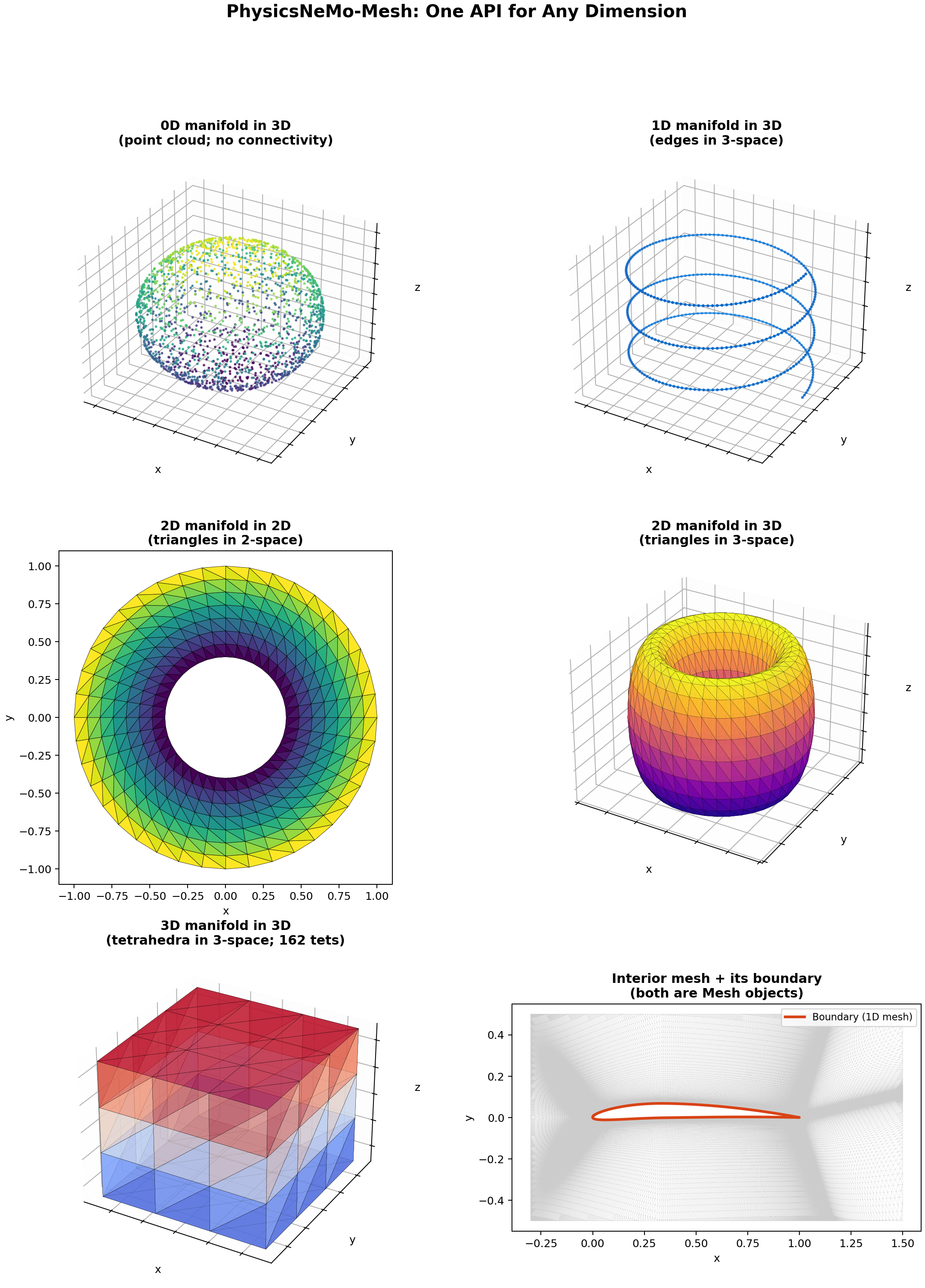
Dimensional Generality

A Mesh data structure is characterized by two dimensions:

• The manifold dimension n_manifold_dims is the intrinsic dimension of each cell. Triangles are 2D, tetrahedra are 3D, edges are 1D, points are 0D.

• The spatial dimension n_spatial_dims is the dimension of the embedding space where vertex coordinates live. A 3D triangle mesh has triangles (2D cells) embedded in 3-space, so n_spatial_dims = 3.

The difference between the two is the codimension:

\[\text{codimension} = n_{\text{spatial\_dims}} - n_{\text{manifold\_dims}}\]

Codimension determines what geometric operations are well-defined. For example, a mesh of codimension 0 (triangles in 2D, tetrahedra in 3D) has no unique normal direction, but its cells fill a region of the embedding space. A mesh of codimension 1 (triangles in 3D, edges in 2D) has a unique normal for each cell. A mesh of codimension 2 or more (edges in 3D) has infinitely many normal directions.

Table 7 Common dimensional configurations

Type	Configuration	Typical use case
Point cloud	Mesh[0, 3]	Lidar scans, particle systems, neural-field query points
Curve in 3D	Mesh[1, 3]	Path planning, fiber bundles, knot theory
2D triangulation	Mesh[2, 2]	2D CFD, planar FEM, image-domain triangulations
Surface mesh	Mesh[2, 3]	CAD geometries, graphics, surface CFD (wall pressure, shear)
Volume mesh	Mesh[3, 3]	3D CFD, structural FEM, full-volume scientific simulations

The Mesh[m, s] subscript notation is a real part of the API: isinstance(mesh, Mesh[2, 3]) returns True for any triangle mesh in 3D. See Dimension-parametrized types later in this chapter.

The Mesh Data Model

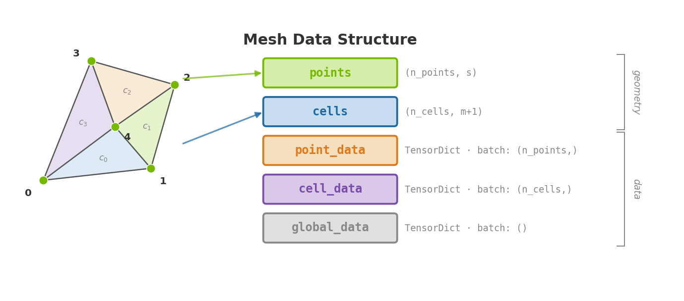
A Mesh is a tensorclass with five fields. Two carry geometry, three carry data:

Mesh(
    points: torch.Tensor,      # (n_points, n_spatial_dims)
    cells: torch.Tensor,       # (n_cells, n_manifold_dims + 1), integer dtype
    point_data: TensorDict,    # Per-vertex data
    cell_data: TensorDict,     # Per-cell data
    global_data: TensorDict,   # Mesh-level data
)

Everything else - centroids, normals, curvature, gradients, neighbors, boundaries - is computed lazily from these five fields and cached.

A minimal example: a triangle in 2D with a couple of attached fields.

import torch
from physicsnemo.mesh import Mesh

### Two tensors define the geometry
points = torch.tensor([[0.0, 0.0], [1.0, 0.0], [0.5, 1.0]])
cells = torch.tensor([[0, 1, 2]])
mesh = Mesh(points=points, cells=cells)

### Attach data of any rank to points, cells, or globally
mesh.point_data["temperature"] = torch.tensor([300.0, 350.0, 325.0])
mesh.point_data["velocity"] = torch.tensor([[1.0, 0.5], [0.8, 1.2], [0.0, 0.9]])
mesh.cell_data["reynolds_stress"] = torch.tensor([[[2.1, 0.3], [0.3, 1.8]]])
mesh.global_data["Re"] = torch.tensor(1.5e6)

print(mesh)

The __repr__ shows the trailing dimensions of each field:

Mesh[n_manifold_dims=2, n_spatial_dims=2](n_points=3, n_cells=1)
    point_data : {temperature: (), velocity: (2,)}
    cell_data  : {reynolds_stress: (2, 2)}
    global_data: {Re: ()}

Why arbitrary-rank tensor fields?

PhysicsNeMo-Mesh stores each field as its own tensor in point_data, cell_data, or global_data, with the rank carried by the tensor shape: a scalar field at vertices has shape (n_points,), a vector field has shape (n_points, n_spatial_dims), a rank-2 tensor field has shape (n_points, n_spatial_dims, n_spatial_dims), and so on.

This matters for physically-consistent PDE surrogates. The solution to a PDE is, in general, a collection of tensor fields of varying rank. A typical fluid simulation has a scalar pressure field, a vector velocity field, and a rank-2 stress tensor field. Solid mechanics adds displacement vectors, strain tensors, and stress tensors.

Different-rank tensors transform differently under symmetries. Under rotation by an orthogonal matrix \(R\), scalars are invariant, vectors transform as \(v' = R v\), and rank-2 tensors as \(T' = R T R^\top\). Under parity (reflection), the picture gets subtler: ordinary vectors flip sign on the reflected components, but pseudovectors like vorticity (the curl of a vector field) flip sign on all components.

Concretely: imagine a fluid simulation around a left-right symmetric airplane in symmetric flow. Given the fields on the left half, what are they on the right? Pressure (scalar) is the mirror image. Velocity (vector) is the mirror image with the cross-flow component flipped sign. Vorticity (pseudovector) is the negative of the mirror image. Three different transformation rules, on the same mesh, on the same physical configuration.

If you flatten everything into a single feature vector [p, vx, vy, vz, ωx, ωy, ωz], you cannot apply different transformation rules to different slots, because the slots have lost their type. Any architecture downstream of that concatenation loses access to spatial equivariance.

Because each field is its own tensor, point_data, cell_data, and global_data carry the per-field rank as part of the tensor shape:

d = mesh.n_spatial_dims

mesh.point_data["pressure"] = torch.zeros(mesh.n_points)     # scalar field
mesh.point_data["velocity"] = torch.zeros(mesh.n_points, d)  # vector field
mesh.cell_data["stress"] = torch.zeros(mesh.n_cells, d, d)   # rank-2 tensor field (matrix)

A model that consumes a Mesh can introspect each field’s shape, infer its rank, and apply the correct transformation. Nested TensorDict keys are available for organizing heterogeneous data (for example, mesh.point_data["boundary_conditions", "inlet", "velocity"]), but the nesting is purely organizational; rank is always carried by the tensor shape.

TensorDict integration and lazy caching

Because Mesh is a tensorclass, it inherits standard TensorDict operations:

• mesh.to("cuda") (or .to(torch.float32)) moves every tensor in the mesh to the target device or dtype in a single call. Nested keys are handled recursively.

• mesh.clone() returns a deep copy with independent storage.

• mesh.save(path) writes a directory tree of memory-mapped tensor files; Mesh.load(path) reads them back. See Serialization for the speed comparison against VTU.

• mesh.pin_memory() pins all tensors for fast asynchronous host-to-device transfer in dataloaders.

Derived geometric quantities (centroids, areas, normals, curvature) are computed on first access and cached automatically:

K_pointwise = mesh.gaussian_curvature_vertices       # computed and cached
areas = mesh.cell_areas                              # computed and cached
centroids = mesh.cell_centroids                      # computed and cached

The cache lives in a separate _cache TensorDict, never mixed with user point_data or cell_data. Because Mesh is intended to be immutable, all operations (transformations, subdivision, repair) return new instances rather than modifying in place - cached values remain valid for the lifetime of the instance. In-place mutation of points or cells (e.g., mesh.points[0] = ...) is unsupported and will silently produce stale cached values. To modify mesh geometry, use the transformation methods (translate, rotate, transform) that return new instances.

Dimension-parametrized types

Mesh supports subscript notation Mesh[manifold_dims, spatial_dims] for type annotations and runtime isinstance checks:

def compute_normals(mesh: Mesh[2, 3]) -> torch.Tensor:
    """Surface normals are only well-defined for codim-1 meshes."""
    return mesh.point_normals

isinstance(mesh, Mesh[2, 3])    # True for triangle meshes in 3D
isinstance(mesh, Mesh[1, ...])  # True for any 1D mesh (any spatial dim)

Mesh[2, 3].boundary             # -> Mesh[1, 3]
Mesh[3, 3].boundary             # -> Mesh[2, 3]

Use ... (Ellipsis) to leave a dimension unconstrained. The .boundary property navigates to the type of the boundary mesh, decrementing the manifold dimension by one.

Symbolic dimension expressions encode the codimension relationship directly:

Mesh["n", "n"]      # any codim-0 mesh
Mesh["n", "n+1"]    # any codim-1 mesh

Simplicial Foundations and the Restriction

The Mesh data model would not work if cells could be arbitrary polygons. The choice to restrict to simplices is what makes the rest of the library possible.

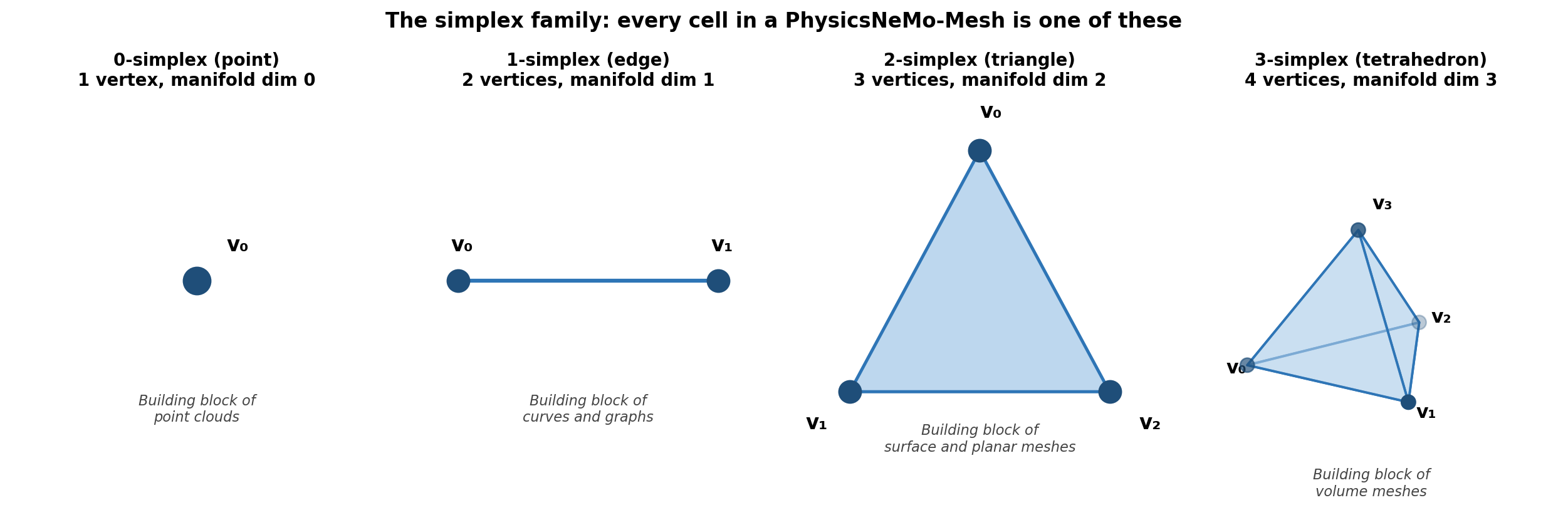
What is a simplex?

A simplex is the natural generalization of a triangle to arbitrary dimensions:

Table 8 The simplex family

n	Common name	Description
0	Point	A single vertex
1	Line segment / edge	Connects 2 points; boundary: 2 points
2	Triangle	Connects 3 points; boundary: 3 edges
3	Tetrahedron	Connects 4 points; boundary: 4 triangles
n	n-simplex	Convex hull of n+1 affinely independent points

A PhysicsNeMo Mesh is a collection of simplices that all share the same n_manifold_dims and share vertices wherever they meet. This is a pure simplicial complex of dimension n.

Why simplicial?

Four key properties depend on the restriction:

Rigorous discrete exterior calculus. Mesh-based discretizations of the gradient, divergence, curl, and Laplacian are well-developed for simplicial meshes (see [Hirani2003] and [Desbrun2005]). Generalizing to arbitrary polygonal or polyhedral meshes is much harder and an open research area.

Dimension-generic algorithms. Because every cell has the same number of vertices (n_manifold_dims + 1), one piece of code computing cell volumes via the Gram determinant works in any dimension without special-casing the cell shape. There is no need for ragged arrays or per-cell-type dispatch.

Vectorization. A rectangular cell tensor enables fully vectorized GPU operations. Mixed-cell-type meshes (a typical VTK file might contain hexahedra, prisms, pyramids, and tetrahedra mixed together) require ragged data structures or per-cell-type loops, both of which kill performance on GPU.

Unambiguous adjacency and boundaries. The boundary of an n-simplex is a union of (n-1)-simplices, and facet-to-cell adjacency is fully determined by the cell tensor. There are no edge cases for non-convex cells, hanging nodes, or T-junctions.

The trade-off

The restriction means Mesh does not natively represent polyhedral cell types you may encounter in CAE pipelines: quadrilaterals and hexahedra (common in structured grids) and pyramids, prisms, and wedges (used near boundaries in CAE solvers). This is a deliberate design trade-off: the simplicial restriction is what enables the vectorization, dimension-generic algorithms, and unambiguous adjacency described above.

In practice, this usually does not block ML mesh workflows, for three reasons:

1. Most ML models do not need full cell geometry for the interior. Point-cloud-based and graph-based architectures need vertex positions and connectivity, not the cell shapes themselves. You can represent a polyhedral interior as a point cloud (Mesh[0, 3]) or an edge graph (Mesh[1, 3]), both of which are well-posed regardless of the source mesh’s cell types. from_pyvista(pv_mesh, manifold_dim=1) does exactly this: it extracts all unique edges from the polyhedral topology to build a vertex graph. DomainMesh only requires that the interior is semantically “inside” the boundary - a point cloud or edge-graph interior is fine.

2. Surface and boundary meshes are typically already triangulated. In cases where they are not (e.g., quad-dominated surface formats), simple splitting works. from_pyvista handles this automatically for manifold_dim=2.

3. Where you do need cell-level structure, derived representations are available. For example, you can build the dual graph (mesh.to_dual_graph()) to get a Mesh[1, 3] where each point is a cell centroid and each edge represents a shared facet, with facet areas and normals stored as edge data.

Mesh is an opinionated format designed for ML mesh workflows. It is not a drop-in replacement for general-purpose mesh I/O libraries, and the simplicial restriction is part of what enables the rest of the design.

When you do triangulate a polyhedral mesh, from_pyvista handles it automatically:

import pyvista as pv
from physicsnemo.mesh.io import from_pyvista

pv_mesh = pv.read("solver_output.vtu")  # mixed cell types
mesh = from_pyvista(pv_mesh)            # auto-triangulated

Note

Triangulation changes the discretization slightly. A hexahedral cell is typically split into 5 or 6 tetrahedra, and the choice affects discrete operator weights. If you are using Mesh for purposes where the discretization matters (e.g., computing differential operators on the triangulated volume), verify that the triangulation does not introduce unwanted error.

Validation

At construction, Mesh validates structural invariants: points is 2D, cells is 2D with integer dtype, n_manifold_dims <= n_spatial_dims, points and cells are on the same device, and the leading dimension of each point_data / cell_data field matches n_points / n_cells (enforced by TensorDict batch size).

For deeper integrity checks - out-of-bounds cell indices, degenerate cells, duplicate vertices, manifoldness - call mesh.validate():

report = mesh.validate()                    # returns a dict of results
mesh.validate(raise_on_error=True)          # raises ValueError on first issue

The boundary of a mesh is also a mesh

The boundary of an n-dimensional simplicial mesh is naturally an (n-1)-dimensional mesh of the same spatial dimension. Mesh.get_boundary_mesh() returns it as a fresh Mesh:

from physicsnemo.mesh.primitives.volumes import cube_volume

volume = cube_volume.load(subdivisions=3)   # Mesh[3, 3]: tetrahedra in 3D
surface = volume.get_boundary_mesh()         # Mesh[2, 3]: triangles in 3D
curve = surface.get_boundary_mesh()          # Mesh[1, 3]: edges in 3D
                                             # (empty for closed surfaces)

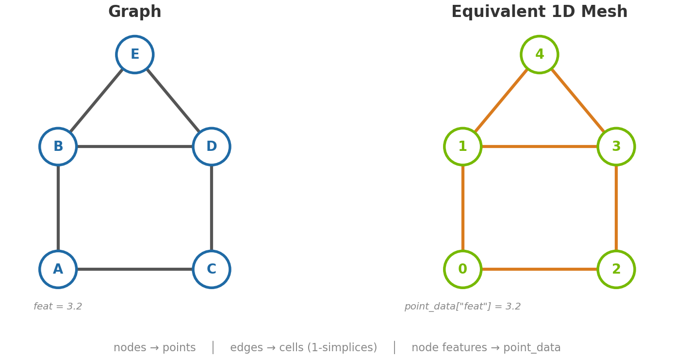
Graphs, Point Clouds, and Geometric Embedding

A 1-simplex is an edge. So a Mesh[1, n_spatial_dims] is, structurally, a graph: its points are nodes, its cells (pairs of point indices) are undirected edges, and point_data / cell_data carry per-node and per-edge features respectively.

Table 9 Graph-mesh correspondence

Graph concept	Mesh equivalent
Node	Point (row of points)
Edge	Cell (row of cells)
Node feature vector	point_data fields
Edge feature vector	cell_data fields

The Mesh[0, 3] and Mesh[1, 3] rows in the dimensional configurations table above are precisely these cases: a point cloud and an edge graph.

Geometric embedding

The distinction between a Mesh[1, n] and an abstract graph \(G = (V, E)\) is that the mesh is a geometric embedding of the graph. An abstract graph is purely combinatorial: it has nodes and edges, but no notion of where nodes are in space, how long an edge is, or what area is associated with a node. (For example, a social network graph has “friendship” edges, but edge length and node area are meaningless concepts.)

A Mesh[1, n_spatial_dims] assigns each vertex a position in \(\mathbb{R}^n\). This embedding induces metric structure on the combinatorial skeleton:

• Edges acquire lengths: \(\ell_{ij} = \|p_i - p_j\|\).

• Dual cells around each vertex acquire areas (or volumes, in higher spatial dimensions).

• The gradient along an edge becomes the scaled difference quotient \((f_j - f_i) / \ell_{ij}\).

• Discrete divergence, Laplacian, and the rest of the DEC machinery follow from the embedding.

Graph libraries like PyTorch Geometric provide abstract graphs. PhysicsNeMo-Mesh provides graphs embedded in geometric space. When your data is inherently spatial - CFD, structural mechanics, weather - the geometric embedding is where much of the physical information lives. Cell areas, normals, curvatures, intrinsic versus extrinsic gradients, and discrete differential operators are all properties of the embedding, not of the combinatorial graph.

For PDE surrogates, keeping data in mesh form as deep into the pipeline as possible preserves access to these geometric quantities (cell areas for finite-volume integration, surface normals for boundary-condition encoding, curvatures as surface features). These are often among the most informative inputs for physically-consistent models.

Point clouds

A Mesh[0, n_spatial_dims] is the degenerate case: vertices with positions but no connectivity. You get one directly by omitting cells at construction time:

cloud = Mesh(points=torch.randn(1000, 3))   # Mesh[0, 3]

There is no edge-derived metric structure, but spatial positions still enable BVH construction, nearest-neighbor queries, surface sampling, and barycentric interpolation. Per-point features live in point_data; the cells tensor is empty.

References

[Hirani2003]

Hirani, A. N. (2003). Discrete exterior calculus (Doctoral dissertation, California Institute of Technology).

[Desbrun2005]

Desbrun, M., Hirani, A. N., Leok, M., & Marsden, J. E. (2005). Discrete exterior calculus. arXiv preprint math/0508341.