Using Mesh

Hands-on walkthroughs of the patterns below live at examples/minimal/mesh/ in the PhysicsNeMo repository (tutorials 1-6). For function- and class-level signatures, see the API reference.

Many of these operations run 10-100x faster on GPU than their CPU equivalents. This speedup makes it practical to run mesh preprocessing inside the training loop rather than as an offline step - and even to embed mesh operations within the model forward pass for end-to-end differentiability. For the full picture on training-time preprocessing, see Mesh in ML Pipelines.

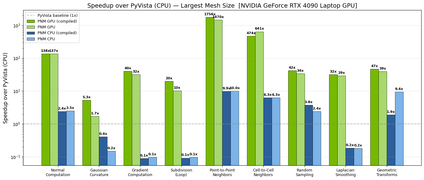
Fig. 14 Per-operation speedup of GPU PhysicsNeMo-Mesh (green) over CPU PyVista (blue) on an NVIDIA GeForce RTX 4090 Laptop GPU. Darker shades show torch.compile-d variants.

Feature Overview

The tables below summarize what is available, grouped by capability. Each group links to the corresponding API page.

Core data structure

See physicsnemo.mesh.mesh.

Capability	Notes
n-dimensional simplicial meshes	Arbitrary manifold and spatial dimensions
Point, cell, and global data containers	Nested TensorDict with arbitrary-rank fields
Memory-mapped serialization	Mesh.save() / Mesh.load() to *.pmsh directories
Mesh merging	Concatenate multiple meshes

Discrete calculus

See physicsnemo.mesh.calculus.

Capability	Notes
Gradient, divergence	LSQ (general-purpose) and DEC (rigorous discrete identities)
Curl	LSQ; 3D only
Laplacian	DEC, with cotangent weights
Intrinsic vs extrinsic derivatives	Tangent space vs ambient space, on embedded manifolds

Geometry and curvature

See physicsnemo.mesh.geometry and physicsnemo.mesh.curvature.

Capability	Notes
Cell areas, volumes, centroids	Gram determinant method, dimensionally generic
Cell and point normals	Generalized cross product (cell); angle-area-weighted (point)
Gaussian curvature	Angle defect method
Mean curvature	Cotangent Laplacian

Topology and adjacency

See physicsnemo.mesh.boundaries and physicsnemo.mesh.neighbors.

Capability	Notes
Boundary and facet extraction	Returns the boundary as a Mesh of one lower dimension
Watertight and manifold checks	is_watertight(), is_manifold()
Adjacency: point-points, point-cells, cell-cells, cell-points	Sparse (offsets, indices) encoding; expand_to_pairs() for COO format

Spatial queries and sampling

See physicsnemo.mesh.spatial and physicsnemo.mesh.sampling.

Capability	Notes
BVH construction and traversal	GPU-accelerated
Point containment, nearest cell	Per-query-point answers from a built BVH
Barycentric interpolation	Sample any field at arbitrary query points
Random point sampling on cells	Dirichlet-distributed barycentric coordinates within each cell

Mesh surgery

See physicsnemo.mesh.subdivision, physicsnemo.mesh.smoothing, physicsnemo.mesh.remeshing, and physicsnemo.mesh.repair.

Capability	Notes
Subdivision	Linear (midpoint), Loop (C² smooth), Butterfly (interpolating)
Laplacian smoothing	Optional feature preservation
Uniform remeshing	Clustering-based; dimension-agnostic
Cleanup (mesh.clean())	Merges duplicate points, removes duplicate cells, drops unused vertices
Quality metrics	Aspect ratio, edge ratios, angles

Transformations

See physicsnemo.mesh.transformations.

Capability	Notes
Translate, rotate, scale	Rotate: angle in 2D; angle-axis in 3D
Arbitrary linear transform	mesh.transform(matrix); works in any dimension

Projections

See Transformations and Projections.

Capability	Notes
Project	Drop spatial dimensions (e.g. 3D to 2D)
Embed	Add spatial dimensions (e.g. 2D to 3D)
Extrude	Increase manifold dimension by one (e.g. surface to volume)

I/O and visualization

See physicsnemo.mesh.io and physicsnemo.mesh.visualization.

Capability	Notes
PyVista interop	from_pyvista() / to_pyvista(); supports STL, VTK, PLY, OBJ, …
Renderers	Interactive PyVista (3D); matplotlib (2D / static 3D)
Scalar coloring	Auto L2-norm for vector fields

Working with Meshes

Creating meshes

Four common ways to create a Mesh.

1. Directly from tensors. Useful for synthetic problems and tests:

import torch
from physicsnemo.mesh import Mesh

points = torch.tensor([
    [0.0, 0.0],
    [1.0, 0.0],
    [1.0, 1.0],
    [0.0, 1.0],
])
cells = torch.tensor([
    [0, 1, 2],
    [0, 2, 3],
])
mesh = Mesh(points=points, cells=cells)

2. From the built-in primitives library. Organized by category (surfaces, volumes, planar, curves, procedural, pyvista_datasets):

from physicsnemo.mesh.primitives.surfaces import sphere_icosahedral, torus
from physicsnemo.mesh.primitives.volumes import cube_volume
from physicsnemo.mesh.primitives.curves import helix_3d

sphere = sphere_icosahedral.load(radius=1.0, subdivisions=3)
donut = torus.load(major_radius=1.0, minor_radius=0.3)
cube = cube_volume.load(subdivisions=2)
helix = helix_3d.load(n_points=200, n_turns=4)

3. From a PyVista mesh. Handles every format PyVista supports (STL, VTK, VTU, VTP, PLY, OBJ, …) and triangulates non-simplicial cell types automatically:

import pyvista as pv
from physicsnemo.mesh.io import from_pyvista

pv_mesh = pv.read("path/to/geometry.stl")
mesh = from_pyvista(pv_mesh)

4. From a saved ``*.pmsh`` directory. See Serialization below.

Device management

A single .to() call moves the entire mesh - geometry, every nested data field, every cached property - to the target device or dtype:

mesh_gpu = mesh.to("cuda")
mesh_fp64 = mesh.to(torch.float64)
mesh_back = mesh_gpu.to("cpu")

mesh.pin_memory() is also available for fast asynchronous host-to-device transfers in dataloaders.

Visualization

mesh.draw() provides one-line visualization with automatic backend selection: matplotlib for 2D, PyVista for 3D. Override with backend="matplotlib" or backend="pyvista".

### Color by a point scalar field
mesh.draw(point_scalars="temperature", cmap="RdBu", show_edges=True)

### Color by a cell scalar field
mesh.draw(cell_scalars="pressure", cmap="viridis")

### Vector fields are auto-converted to L2-norm for coloring
mesh.draw(point_scalars="velocity", cmap="turbo")

In Jupyter notebooks, the PyVista backend supports interactive widgets via pv.set_jupyter_backend("trame"). draw() returns the plotter / axes object so you can customize before display.

Transformations

Geometric transformations are pure functions: they return a new mesh and leave the original unchanged.

import numpy as np

mesh_translated = mesh.translate([1.0, 0.0, 0.0])
mesh_rotated = mesh.rotate(angle=np.pi / 4, axis=[0, 0, 1])
mesh_scaled = mesh.scale(2.0)                      # uniform
mesh_anisotropic = mesh.scale([2.0, 1.0, 0.5])     # per-axis

By default, transformations affect only the geometry (the points tensor); attached field data is left unchanged. This is correct for scalar fields like temperature (invariant under rotation) but wrong for vector fields like velocity. Opt in to co-rotation via the transform_*_data flags:

mesh_rotated = mesh.rotate(
    angle=np.pi / 4,
    axis=[0, 0, 1],
    transform_point_data={"velocity": True},
    transform_global_data={"U_inf": True},
)

Pass True to transform all compatible fields, or a dict / TensorDict selecting specific fields. DomainMesh uses the same flags to propagate transforms across an entire simulation domain.

Note

In dimensions higher than 3, the angle-axis rotate formulation does not generalize. Use mesh.transform(matrix) directly with an arbitrary orthogonal matrix instead.

Topology and adjacency

### Boundaries and facets
boundary = mesh.get_boundary_mesh()      # the (n-1)-D outer boundary
facets = mesh.get_facet_mesh()           # all (n-1)-D simplices, including interior
is_closed = mesh.is_watertight()
is_manifold = mesh.is_manifold()

### Adjacency queries (returned as sparse offset/index arrays)
point_neighbors = mesh.get_point_to_points_adjacency()
cell_neighbors = mesh.get_cell_to_cells_adjacency()

The adjacency objects use a sparse (offsets, indices) encoding. Convert when you need a different representation:

neighbors_list = point_neighbors.to_list()                     # ragged list-of-lists
src, tgt = point_neighbors.expand_to_pairs()                   # (E,), (E,)
edge_index = torch.stack([src, tgt], dim=0)                    # PyG COO format: (2, E)

Discrete calculus: DEC vs LSQ

Two complementary methods for discrete differential operators:

• Discrete Exterior Calculus (DEC) is a mathematically rigorous framework where the discrete operators satisfy exact discrete versions of classical theorems (Stokes, Gauss-Bonnet, Helmholtz decomposition). It uses cotangent weights and circumcentric dual cells. See [Hirani2003] and [Desbrun2005].

• Weighted least-squares (LSQ) is the practical CFD/FEM workhorse. Gradients are reconstructed by fitting a linear function to neighboring values; the result is exact for linear fields and first-order accurate in general.

Use DEC when you need exact discrete identities or are working with surface PDE solvers where the Laplace-Beltrami operator is the natural choice. Use LSQ for general-purpose CFD/FEM-style preprocessing where robustness on arbitrary topology matters more than exact discrete identities.

### Compute gradient of "pressure" via least-squares (default)
mesh = mesh.compute_point_derivatives(keys="pressure", method="lsq")
grad_p = mesh.point_data["pressure_gradient"]      # shape (n_points, n_spatial_dims)

### Same with DEC (Discrete Exterior Calculus), for an intrinsic gradient
mesh = mesh.compute_point_derivatives(keys="pressure", method="dec")

For surfaces, you can choose between intrinsic (tangent-space) and extrinsic (ambient-space) derivatives:

mesh = mesh.compute_point_derivatives(keys="T", gradient_type="intrinsic")
mesh = mesh.compute_point_derivatives(keys="T", gradient_type="extrinsic")

For the underlying mathematics, see the physicsnemo.mesh.calculus API reference.

Differential geometry

Curvature, normals, and tangent spaces are exposed as cached properties.

normals = mesh.point_normals                         # (n_points, n_spatial_dims)
K = mesh.gaussian_curvature_vertices                 # (n_points,)
H = mesh.mean_curvature_vertices                     # (n_points,)

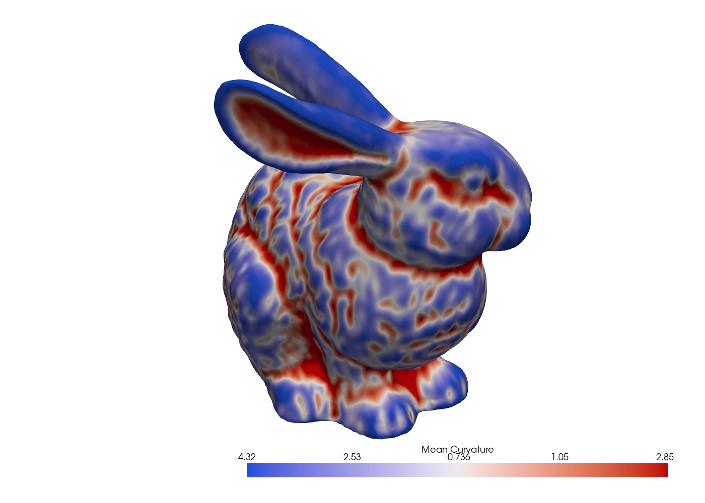
Fig. 15 Mean curvature on the Stanford bunny via the cotangent Laplacian.

See the geometry and curvature API references for the full list of available properties and functions.

Spatial queries

For point-in-mesh queries, nearest-cell searches, and barycentric interpolation, build a Bounding Volume Hierarchy once and reuse it for many queries:

from physicsnemo.mesh.spatial import BVH
from physicsnemo.mesh.sampling import find_containing_cells

bvh = BVH.from_mesh(mesh)

### BVH gives fast approximate candidates (AABB overlap)
query_points = torch.rand(1000, 3)
candidates = bvh.find_candidate_cells(query_points)

### Exact containment uses barycentric coordinate testing
cell_indices, bary_coords = find_containing_cells(mesh, query_points)

### Or sample any field at the query points (barycentric interpolation)
sampled = mesh.sample_data_at_points(query_points, data_source="points")

Mesh surgery

Subdivision, smoothing, remeshing, and repair return new meshes:

### Subdivision
refined = mesh.subdivide(levels=2, filter="linear")    # midpoint, no smoothing
smooth = mesh.subdivide(levels=2, filter="loop")       # C² smooth
interp = mesh.subdivide(levels=2, filter="butterfly")  # interpolating

### Smoothing
from physicsnemo.mesh.smoothing import smooth_laplacian
smoothed = smooth_laplacian(mesh, n_iter=10)

### Remeshing: rebuild from scratch with a target cell count
from physicsnemo.mesh.remeshing import remesh
coarse = remesh(mesh, n_clusters=5000)

### Repair: merge duplicate points, deduplicate cells, drop unused vertices
clean = mesh.clean()

For incremental quality fixes (instead of the all-in-one clean()), use the targeted methods in physicsnemo.mesh.repair.

Serialization

By convention, Mesh objects are saved to *.pmsh directories and DomainMesh objects to *.pdmsh directories. Unlike a single-file format such as VTU, each save produces a directory containing one memory-mapped tensor file per leaf field, with subfolders that mirror the mesh’s data structure. This is convenient for data surgery: you can add, drop, or replace individual fields directly on disk without reloading or rewriting the entire mesh.

mesh.save("/path/to/mesh.pmsh")
mesh = Mesh.load("/path/to/mesh.pmsh", device="cuda")

Loading uses byte-for-byte memory mapping with near-zero parsing overhead.

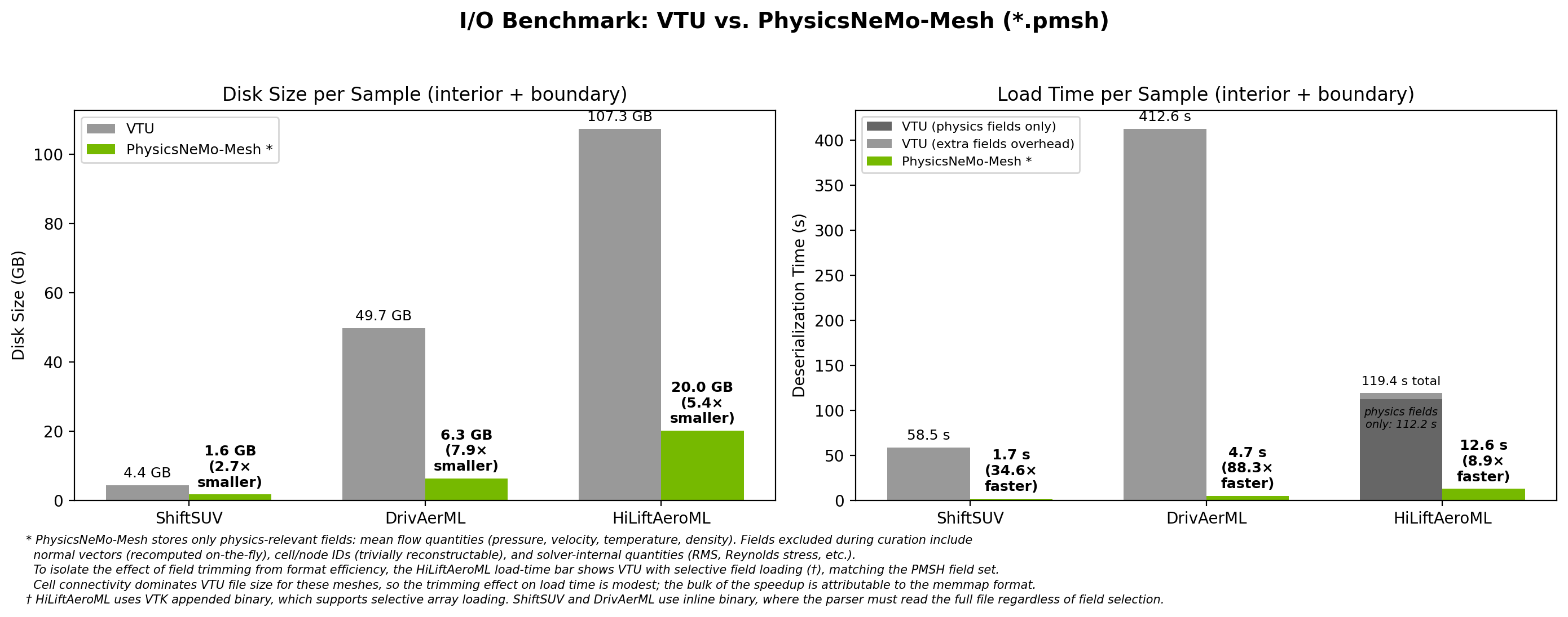
Fig. 16 PMSH is 9x to 88x faster to load than VTU and 3x to 8x smaller on disk across three production CFD datasets.

The speedup comes from two sources: the user stores only the fields they need (rather than the solver’s full output), and the memory-mapped format avoids parsing overhead entirely. save() itself does not drop any fields - it serializes the entire Mesh faithfully. The directory layout also enables partial loading (read just the fields you need) and on-disk surgery (swap a single field without rewriting the whole mesh). See DomainMesh for the same pattern applied to full simulation domains.

torch.compile compatibility

Most operations are torch.compile-compatible, but some patterns cause graph breaks:

• scatter_add_ operations (used in edge counting, facet extraction, adjacency).

• torch.where with variable-length output.

• torch.unique and similar operations with variable-sized outputs.

Three patterns work in practice:

1. Separate preprocessing from inner loops. Wrap mesh-topology computations in non-compiled code:

### Outside compiled region
neighbors = mesh.get_point_to_points_adjacency()

@torch.compile
def compute_laplacian(points, neighbor_indices, neighbor_offsets):
    ...

2. Pre-compute cached properties before entering compiled code. Cached quantities like mesh.cell_areas are computed lazily on first access; the first access inside a compiled function causes a graph break. Touch them once outside first:

_ = mesh.cell_areas        # warm cache
_ = mesh.cell_normals

@torch.compile
def my_loss(mesh):
    ...

3. Use ``mode=”reduce-overhead”`` when graph breaks are unavoidable. This minimizes per-graph-break dispatch cost.

Graph and Point Cloud Conversion

For the conceptual relationship between meshes, graphs, and point clouds - including why a geometrically embedded graph carries more information than an abstract one - see Graphs, Point Clouds, and Geometric Embedding in the Concepts chapter.

For a higher-dimensional mesh, two natural graph representations are available:

• The edge graph (the 1-skeleton) treats mesh vertices as nodes and mesh edges as edges. Best when data lives on vertices, as in most graph-neural-network surrogates.

• The dual graph treats cell centroids as nodes, with edges between cells that share a facet. Best when data lives on cells, as in finite-volume CFD where fluxes are exchanged at cell-cell interfaces.

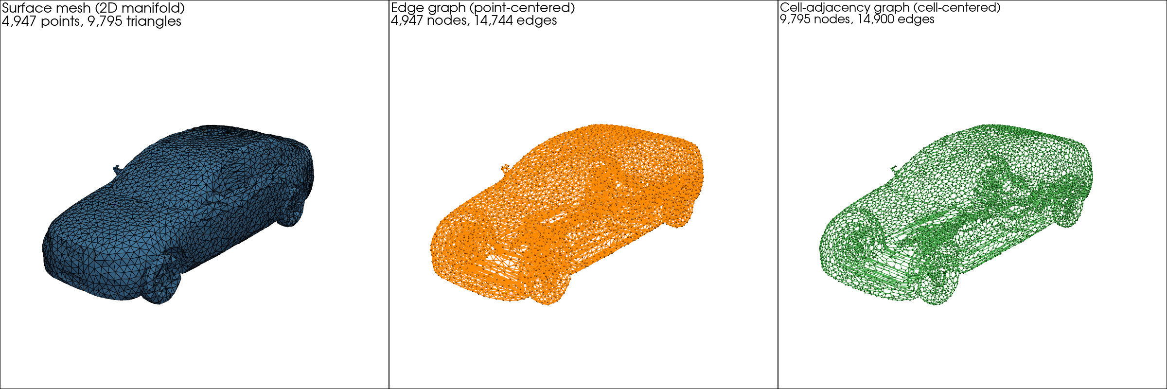
Fig. 17 The DrivAerML car: surface mesh (left), edge graph (center, vertex-centered), and dual graph (right, cell-centered). All three are first-class Mesh objects.

surface = ...                              # Mesh[2, 3]: triangles in 3D

edge_graph = surface.to_edge_graph()       # Mesh[1, 3]: vertex-centered
dual_graph = surface.to_dual_graph()       # Mesh[1, 3]: cell-centered
point_cloud = surface.to_point_cloud()     # Mesh[0, 3]: no connectivity

Each converted result is itself a Mesh and can use any of the operations covered earlier. These conversion methods are documented in the Mesh API reference.

PyTorch Geometric interop

For workflows already built around PyG, adjacency objects convert to edge_index format:

adjacency = mesh.get_point_to_points_adjacency()
src, tgt = adjacency.expand_to_pairs()
edge_index = torch.stack([src, tgt], dim=0)      # shape (2, n_edges)

from torch_geometric.nn import GCNConv
x = mesh.point_data["features"]
y = GCNConv(in_channels=x.shape[-1], out_channels=64)(x, edge_index)