Mesh in ML Pipelines

This chapter covers patterns for using PhysicsNeMo-Mesh in ML training pipelines.

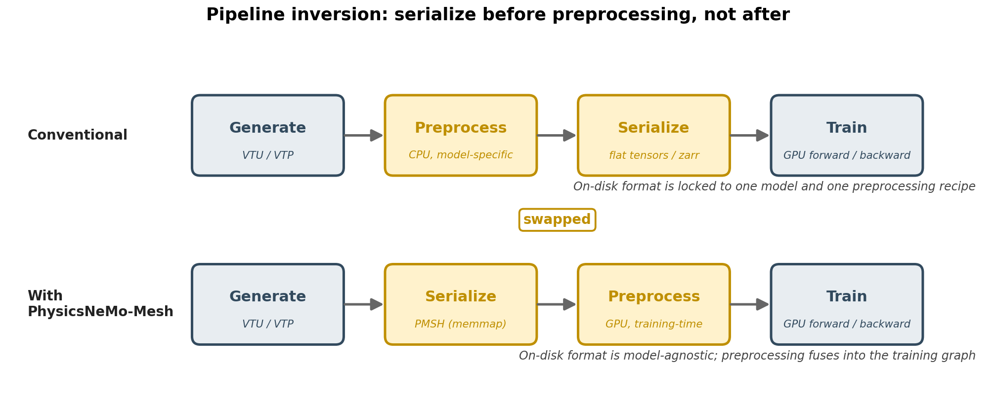
Pipeline Positioning

PhysicsNeMo-Mesh supports a serialize-then-preprocess ordering: convert solver output to the model-agnostic *.pmsh format once, then preprocess on-the-fly at training time on GPU. Because PMSH preserves full mesh structure, the same serialized files can serve any downstream model. Preprocessing is GPU-resident and autograd-compatible, so it can run in parallel with the forward and backward pass and even fuse into a single computational graph.

Training-Time Preprocessing

Preprocessing fuses into the training step, not as a separate offline pass:

from physicsnemo.mesh import Mesh

def training_step(mesh: Mesh, model):
    ### Move to GPU and warm cached properties
    mesh = mesh.to("cuda")
    _ = mesh.cell_areas       # warm cache before any compiled region

    ### Compute derived features at training time
    mesh = mesh.compute_point_derivatives(keys="pressure", method="lsq")

    ### Forward pass: the model consumes the structured mesh
    prediction = model(mesh)
    loss = loss_fn(prediction, mesh.point_data["target"])
    return loss

Standard PyTorch dataloader patterns (num_workers, pin_memory) work unchanged. The next batch’s preprocessing and host-to-device transfers run concurrently with the current batch’s forward and backward pass.

Batching

Different meshes typically have different numbers of points and cells, so they cannot be stacked into a single dense tensor without padding. Two common batching strategies:

Fixed-size padding. Pad every mesh in the batch up to a fixed size chosen to be larger than any expected mesh. Padding masks are stored as boolean tensors so the model can ignore the pad regions. Simplest when batch composition is known in advance.

Power-based padding. Pad up to the next power of two (or some other discrete bucket size). Dramatically reduces the number of unique shape signatures the model sees, which matters for torch.compile shape-specialization caching: instead of recompiling for every distinct batch size, the compiler only sees a small set of bucketed sizes. The trade-off is some memory overhead for padding to the next bucket.

Both strategies are demonstrated in tutorial 6. The right choice depends on how heterogeneous the mesh sizes are in your dataset and whether you are using torch.compile.

Feature Extraction

Keeping mesh structure in the training loop enables computing new features from raw simulation data. A typical example: the DrivAerML dataset provides surface pressure and wall shear stress, but the classic boundary-layer-stability indicator is the streamwise pressure gradient \(dp/ds\), which is not directly available. With the mesh structure available at training time:

from physicsnemo.mesh.io import from_pyvista
import pyvista as pv

mesh = from_pyvista(pv.read("boundary_1.vtp")).to("cuda")

### Convert cell-centered fields to vertex-centered for differentiation
mesh = mesh.cell_data_to_point_data()

### Compute the surface pressure gradient (extrinsic, in 3D space)
mesh = mesh.compute_point_derivatives(
    keys="pMeanTrim", gradient_type="extrinsic"
)

### Combine with the wall shear stress direction
grad_p = mesh.point_data["pMeanTrim_gradient"]                 # (n_points, 3)
wss = mesh.point_data["wallShearStressMeanTrim"]                # (n_points, 3)
wss_hat = wss / wss.norm(dim=-1, keepdim=True).clamp(min=1e-8)
mesh.point_data["adverse_pg"] = (grad_p * wss_hat).sum(dim=-1)

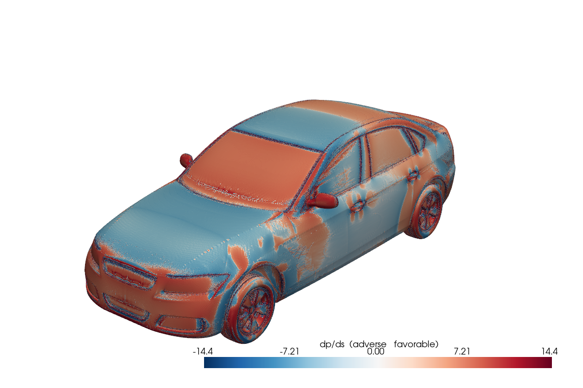
Fig. 19 Adverse pressure-gradient indicator on the DrivAerML car. Red regions are destabilizing; blue is favorable. Computed from raw simulation data at training time.

The pattern is general: load raw data, convert between cell-centered and vertex-centered representations, compute gradients, combine with other fields. Each step is GPU-accelerated and autograd-compatible.

Data Augmentation

For non-equivariant model architectures, augmenting the training data with random rotations, reflections, and translations of the same physical problem is a common way to improve generalization. With DomainMesh, this is a one-line operation that propagates consistently through the interior, every boundary, and the global metadata:

import math
import torch

dm = ...  # DomainMesh loaded or constructed earlier

angle = torch.rand(1).item() * 2 * math.pi
dm_aug = dm.rotate(
    angle=angle,
    transform_point_data={"U": True},
    transform_global_data={"U_inf": True},
)

The transform_*_data flags (covered in Using Mesh) co-rotate vector and tensor fields alongside the geometry. This is sometimes called quasi-equivariance: the model is not structurally equivariant, but training on rotated copies of each sample encourages it to behave approximately equivariantly.

torch.compile compatibility

The graph-breaking patterns and the three working patterns (separate preprocessing from inner loops, pre-compute cached properties, mode="reduce-overhead") are covered in Using Mesh under torch.compile compatibility. They apply equally to standalone preprocessing and to preprocessing fused into a training step.

Future Directions

PhysicsNeMo-Mesh is the first step in a data → layers → models progression toward physically-consistent, generalizable PDE surrogates:

• Step 1 (data): PhysicsNeMo-Mesh and DomainMesh provide the semantics-rich data layer. This step is available today and works with any model architecture. For how to get your data into Mesh format, see Creating and loading a Mesh.

• Step 2 (layers) (planned): TensorDict-compatible primitive layers in physicsnemo.nn.layers (linear/MLP, attention, message-passing) that operate directly on nested semantic structure, without forcing an early flatten. An “off-ramp” collapses a TensorDict into a single concatenated tensor in a spatially-invariant manner so that non-equivariant downstream blocks can still consume the data when needed.

• Step 3 (models) (planned): New equivariant architectures built on top of data and layers.

Steps 2 and 3 are a roadmap; adopting Mesh and DomainMesh does not require waiting for them. In the near term, several existing CAE datapipes (DoMINO, Transolver, GeoTransolver, GLOBE) are being refactored to ingest and produce Mesh TensorDicts as a drop-in replacement for CPU-bound PyVista/VTK preprocessing.