CannyEdgeDetector

Overview

The Canny edge detector is a widely used edge detection algorithm in computer vision and image processing. Its purpose is to identify and extract the boundaries of objects within an image by detecting significant intensity changes, which correspond to edges.

Processing Steps

1. Noise Reduction: The input image is first smoothed using a Gaussian filter to reduce noise. This step is not included in this operator.

2. Gradient Calculation: Use Sobel filter to calculate the intensity gradients of the image. Both the magnitude and direction (angle) of the gradient are computed at each pixel.

3. Non-Maximum Suppression: To thin out the edges and retain only the most significant ones, non-maximum suppression is applied. This step keeps only the local maxima in the gradient direction, resulting in one-pixel-wide edges.

4. Double Thresholding: Two thresholds are applied to classify edge pixels as strong, weak, or non-edges.

5. Edge Tracking by Hysteresis: Weak edges are included in the final output only if they are connected to strong edges. This linking process ensures that true edges are preserved while isolated noise-induced responses are discarded.

Implementation Details

Limitations

This implementation supports only U8 images. For the Sobel filter, only kernel sizes of 3x3, 5x5, and 7x7 are available. The output is also a U8 image, containing only the detected edges. Edge tracking by hysteresis utilizes the Connected Component Labeling (CCL) approach, with a maximum of 65,536 labels supported. If this limit is exceeded, the operator returns CUPVA_VPU_APPLICATION_ERROR.

Implementation Structure

The implementation is organized into four memory passes. In the first memory pass, the intensity and direction of image gradients are computed. The second memory pass performs NMS and double thresholding. The third and fourth passes belong to CCL. In the third, the edge type map—classifying pixels as strong-edge, weak-edge, or non-edge—is read and each pixel receives an intermediate label. The label map is stored in a dedicated VMEM super bank, therefore the label map tree is collapsed without additional memory I/O. The fourth memory pass relabels the pixels and generates the final edge map.

To optimize memory usage, VMEM buffers are overlaid between the first two memory passes and CCL using unions. Intermediate results, including gradient intensity, direction and intermediate labels, are written back to main memory. As the first two stages are compute-bound, the latency of reading and writing these intermediate results can be effectively hidden by pipelining DMA transfers and VPU processing. However, in CCL the fourth memory pass is IO bound.

Dataflows

Six RasterDataFlows are used for input, output, and intermediate results. RasterDataFlow can handle cases where the image size is not a multiple of the tile size.

The input raster dataflow pads the image boundary with zeros, with the padding size being the Sobel filter radius. The input image tiles are stored in a circular buffer in VMEM, reducing the computation of overlapped halo between tiles.

In the second memory pass, the input gradient intensity should be padded using boundary pixel extension (BPE) padding mode, with a padding size of 1. The input gradient intensity tiles are also stored in a circular buffer in VMEM. The input gradient direction has no halo, explicitly setting the halo size to 0 and the region of interest (ROI) to the image rounded up to multiples of tiles. When the image size is not a multiple of tiles, the tail tile in a tile row or column is padded with zeros, which represent the horizontal direction. So that these padded pixels do not affect the NMS results for valid image pixels in the tail tiles.

In the CCL stage, both the input edge type map and the intermediate label image are padded horizontally, with 64 pixels added to each side and a padding value of 0. Due to a -2 row skew in the intermediate label image, the valid width becomes the image width plus 64. As a result, the region of interest (ROI) for the input intermediate label image raster dataflow starts at an x offset of 64.

Five output raster dataflows are employed. When the image dimensions are not exact multiples of the tile size, the write triggers may not suffice. To address this, three output raster dataflows are linked together, allowing them to share channels and write triggers.

ICache Prefetch

The code size exceeds the 16KB ICache capacity, so ICache prefetch is invoked twice, each time prefetching 8KB of instruction code which is half the cache capacity. The first prefetch occurs before the first stage execution loop, and the second before the CCL execution loop. Instruction sequences are carefully arranged in the BCF file according to their execution order. Starting with PVA SDK 2.6.0, the build system defaults to the ASIP programmer’s Clang frontend. Accordingly, the LLVM-version BCF file or the Noodle-version BCF file is selected, depending on the PVA SDK version in use.

Output Demo

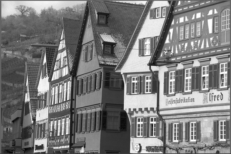
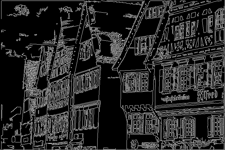
Although this operator does not include edge tracking by hysteresis, the output below shows the detected edges produced by combining this operator with the reference implementation of edge tracking by hysteresis. The image on the left is the input, while the image on the right shows the corresponding detected edges. The threshold for strong edges is 300 and the threshold for weak edges is 100.

Figure 1: Sample input image (left) and output results (right).

Performance

Execution Time is the average time required to execute the operator on a single VPU core. Note that each PVA contains two VPU cores, which can operate in parallel to process two streams simultaneously, or reduce execution time by approximately half by splitting the workload between the two cores.

Total Power represents the average total power consumed by the module when the operator is executed concurrently on both VPU cores. Idle power is approximately 7W when the PVA is not processing data.

For detailed information on interpreting the performance table below and understanding the benchmarking setup, see Performance Benchmark.

ImageSize	DataType	KernelSize	TestData	Execution Time	Submit Latency	Total Power
1920x1080	U8	3x3	baboon	7.219ms	0.027ms	11.257W
1920x1080	U8	5x5	baboon	5.536ms	0.028ms	11.939W
1920x1080	U8	7x7	baboon	5.407ms	0.028ms	11.939W

Reference

[1] https://docs.opencv.org/4.x/da/d22/tutorial_py_canny.html