PeakDetection#

Overview#

Peak detection [1] is a fundamental signal processing algorithm used in RADAR systems to identify and locate targets in the Range-Doppler map. The algorithm uses Non-Maximum Suppression (NMS) on Non-Coherent Integration (NCI) data to detect local maxima that represent estimated targets. When a local maximum is found, the algorithm searches for the most probable TX antenna within the NCI data over RX channels. The peak detection algorithm is particularly important in automotive radar applications where it serves as a critical step in the radar signal processing pipeline, enabling the identification of potential targets such as vehicles, pedestrians, and other objects in the environment.

Algorithm Description#

Since there are multiple variants of the peak detection algorithm, the scheme used is described as follows:

It uses Doppler Division Modulation (DDM) instead of Time Division Modulation (TDM).
The peak detection’s input consists of:
1. FT2D, Range-Doppler map over RX antennas
2. nciRx, unfolded Range-Doppler map, which is the NCI combined Range-Doppler map over RX antennas
3. nciFinal, folded Range-Doppler map, which is accumulated over Doppler folds
4. noise, estimated noise, which is per range bin
The output includes: the total number of detected peaks, per detected peak’s range index, folded Doppler index, unfolded Doppler index, and the snapshot of FT2D with all TX and RX channel combinations.

The Python code is described as follows:

import numpy as np

# Nb - number of range bins (samples)
# Nr - number of Doppler bins (ramps)
# NofTx - number of TX antennas
# RepeatFold - number of Doppler folds
# DDMspace - pattern of the Doppler Division Modulation
for ibin in range(1, Nb - 1):
   for ifold in range(Nr // RepeatFold):
      # if the current value is a local maximum and
      # the value is larger than the noise threshold
      if nciFinal[ibin, ifold] > noise[ibin]:
         # if the current value is larger than the left and right neighbors
         if (nciFinal[ibin, ifold] > nciFinal[ibin - 1, ifold] and
            nciFinal[ibin, ifold] > nciFinal[ibin + 1, ifold]):
            PreiFold = (ifold - 1) % (Nr // RepeatFold)
            PostiFold = (ifold + 1) % (Nr // RepeatFold)
            if (nciFinal[ibin, ifold] > nciFinal[ibin, PreiFold] and
               nciFinal[ibin, ifold] > nciFinal[ibin, PostiFold]):
               # Peak found, increase peak counter and store values
               Peak['N'] += 1
               Peak['DET'].append({
                  'Rind': ibin,
                  'DFoldind': ifold,
                  'Dind': None,
                  'Snap': None,
               })

               # Search the first TX antenna's peak position in the Doppler domain
               candi = np.zeros(RepeatFold)
               for iCand in range(RepeatFold):
                  colIdx = (DDMspace + ifold + (Nr / RepeatFold * iCand - 1)+1) % Nr
                  candi[iCand] = np.sum(nciRx[ibin, colIdx.astype(int)])

               maxValue = np.max(candi)
               mi = np.argmax(candi)

               # Calculate and store Doppler index of the first TX antenna
               Peak['DET'][-1]['Dind'] = (ifold + (Nr / RepeatFold * mi)) % Nr

               # Loop over TX antennas and store Range-Doppler map values
               # at peak location for all RX antennas
               snapValues = []
               for iss in range(NofTx):
                  col_idx = (DDMspace[iss] + ifold + (Nr / RepeatFold * mi)) % Nr
                  # get Range-Doppler map value at peak location of all RX channels
                  snapValues.extend(FT2D[ibin, :, col_idx])
               Peak['DET'][-1]['Snap'] = np.array(snapValues)

Notes:

The first and last bins within the range direction are skipped when traversing nciFinal.
The NMS compares the up, down, left, and right bins.
If the candidate bin is the first bin within the Doppler direction, then NMS selects the last bin with the same range index as its left neighbor. This also applies to the last bin within the Doppler direction. This leverages the periodic property of the FFT (Fast Fourier Transform) in the Doppler direction.

Design Requirements#

The number of unfolded Doppler bins supports either 512 or 1024, and the repeat fold is fixed at 8.
The number of range bins must be a multiple of tile height.
Both the number of TX and RX antennas are fixed at 4.

Implementation Details#

NMS Step#

Since the supported number of folded Doppler bins is either 64 or 128 and PVA has a width of 16 uint32_t elements per double vector instruction, setting the tile width to match the width of nciFinal ensures a reasonable number of instructions for further loop unrolling and software pipelining. To reduce the fetching cost of border bins in the opposite range direction, the HALO width is deliberately set to 1. Filling these HALO bins is handled on the VPU side. Agen is used to further reduce the cost of pointer arithmetic. Overall, an RDF dataflow with a HALO size of 1 is used, similar to normal 3x3 NMS filtering.

The first and last range bins are skipped in the NMS step. This is implemented by setting the corresponding estimated noise to the maximum value of uint32_t, so that the first and last range bins will not survive after comparing with the noise threshold. Otherwise, extra code paths would be needed to handle this specific case.

The output of the NMS step is no longer tile-sized bins, but the range and folded Doppler indices (i.e., coordinates of non-zero bins within nciFinal). Also, the number of outputs within a tile is not fixed and will affect the procedures in the next steps. Last but not least, the NMS step is compute-bound after adding these additional operations.

Unfolded Doppler Index Step and Snapshot Data Step#

For the unfolded Doppler index step, it is conceptually needed to fetch multiple times when traversing all the possible DDM positions within the nciFinal. However, it is equivalent to fetch all bins with that specific range index from DRAM to VMEM once, then extract the corresponding elements using DDM positions, which saves the per-DMA read latency. Once the unfolded Doppler index has been calculated, in the snapshot data step, it calculates a set of TX * RX offsets within nciFinal. Then GSDF dataflow is used to fetch these bins.

The computation part in these two steps is simple. The main challenge here is that the number of indices per tile is not fixed. And a 1000 maximum number of peaks cannot be fitted into one VMEM. Therefore, the current implementation uses a local peak buffer within one VMEM and accumulates the output of NMS and judges whether the buffer’s usage exceeds some threshold that requires calculating the unfolded Doppler index and snapshot data, then transfers the result to DRAM. Apparently, this changes the device side’s processing flow, since originally PVA can finish the NMS operations among all tiles and then perform the following steps. The processing flow is shown in the following figure:

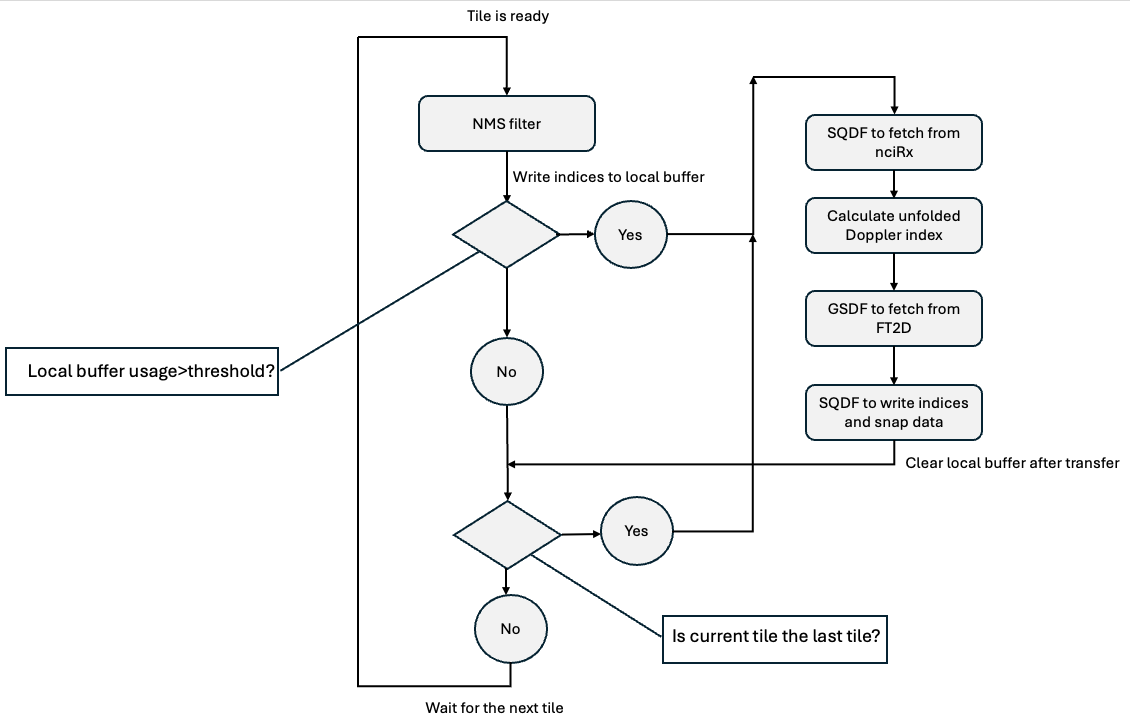
Peak Detection Device Side Processing Flow — Figure 1: Peak Detection’s Device Side Processing Flow#

There is no peak number limitation on the device side after using the above processing flow. Conceptually, the unfolded Doppler index step and snapshot data step can be computed sequentially, but the current implementation interleaves these operations on a per peak basis. This is based on the following reasons:

The amount of data to be read from and written to DRAM is so small that DMA performance is bound to its latency instead of bandwidth.
It is independent between the detected peaks.
Gathering data in the snapshot data step takes 90% of the time consumption among these steps.

After these, the unfolded Doppler index step and transfer output to DRAM operations are interleaved with the gathering data step.

Performance#

The time consumption can be decomposed into two parts:

The NMS step, which is compute-bound and proportional to the dimension of nciFinal.
Both the unfolded Doppler index step and snapshot data step are memory-bound and proportional to the number of detected peaks.

The test cases for profiling use nciFinal with 224 range bins and 64 Doppler bins, and the number of detected peaks is less than 100.

Execution Time is the average time required to execute the operator on a single VPU core. Note that each PVA contains two VPU cores, which can operate in parallel to process two streams simultaneously, or reduce execution time by approximately half by splitting the workload between the two cores.

Total Power represents the average total power consumed by the module when the operator is executed concurrently on both VPU cores. Idle power is approximately 7W when the PVA is not processing data.

For detailed information on interpreting the performance table below and understanding the benchmarking setup, see Performance Benchmark.

FilePostfix	Execution Time	Submit Latency	Total Power
1	0.160ms	0.031ms	10.392W

Reference#

M. O. Kolawole, “Radar Systems, Peak Detection and Tracking”, Elsevier, Oxford, 2003.