DOA (Direction Of Arrival) and Target Processing#
Overview#
Direction of Arrival (DOA) is a fundamental radar signal processing technique that estimates the angular position (azimuth and elevation) of detected targets relative to the radar sensor. By analyzing phase and amplitude differences across multiple receive antenna elements in a MIMO (Multiple-Input Multiple-Output) radar array, the DOA algorithm determines where targets are located in 3D space, complementing range and velocity measurements from earlier processing stages. The DOA algorithm represents a sophisticated implementation of interferometric angle estimation, combining the precision of phase-based methods with the computational efficiency of FFT processing, making it well-suited for real-time radar applications. The algorithm is based on the following principles:
Interferometric Phase Measurement: The algorithm measures the phase difference between signals received by two or more antennas, which is directly proportional to the target’s angle of arrival.
FFT-Based Angle Estimation: The phase difference is converted into a frequency domain representation using FFT, allowing for efficient angle estimation.
Angular Resolution: The algorithm achieves high angular resolution through spatial FFT processing across the antenna array aperture, with resolution determined by the array length and operating wavelength.
Computational Efficiency: The algorithm is designed to be computationally efficient, making it suitable for real-time applications.
Algorithm Description#
FFT-based angle estimation is a sophisticated radar signal processing technique used for Direction of Arrival (DOA) estimation to determine the angular position of detected targets.. Here’s a comprehensive overview:
1. Fundamental Principle#
Spatial Sampling Principle
Antenna Array:      [Ant1] --d--> [Ant2] --d--> [Ant3] --d--> [Ant4]
                        ↓            ↓            ↓            ↓
Received Signals:    s₁(t)        s₂(t)        s₃(t)        s₄(t)

Key Relationship:
θ (angle) → Δφ (phase shift) → Δt (time delay)

Δφ (Phase Shift): The phase difference that results from the time delay.
Δt (Time Delay): The time difference between when the signal arrives at adjacent antenna elements.
These relationships form the basis for angle estimation.
Time Delay Relationship:
- where:
\(d\) = element spacing
\(c\) = speed of light
Phase Shift Relationship:
- where:
\(λ\) = wavelength
Core Concept: Multiple antenna elements spaced at regular intervals sample the spatial wavefront, creating a spatial signal that can be analyzed using FFT.
2. Mathematical Foundation#
FFT-based angle estimation leverages the direct relationship between spatial frequencies in the FFT domain and physical angles of arrival.
Spatial Frequency Domain
The FFT transforms spatial array samples into a spatial frequency spectrum. The relationship between spatial frequency and angle is bidirectional:
The spatial frequency \(k\) is given by:
- where:
\(k\) - spatial frequency (cycles per wavelength)
\(d\) - antenna element spacing (meters)
\(λ\) - signal wavelength (meters)
\(θ\) - angle of arrival (radians)
Angle Extraction from FFT Output
Each FFT bin index corresponds to a specific angle of arrival. The mapping is given by:
- where:
\(n\) - FFT bin index relative to zero frequency (center bin)
\(N\) - total number of FFT points
\(θ\) - estimated angle of arrival (radians)
This direct mapping enables efficient angle estimation by identifying peak locations in the FFT spectrum and converting bin indices to angles using the formula above or a pre-computed lookup table.
Angular Resolution
The theoretical angular resolution of the FFT-based method is determined by the array aperture:
where \(L\) is the total array aperture length and \(N_{elements}\) is the number of physical antenna elements.
3. Algorithm Workflow#
The algorithm follows this processing pipeline:
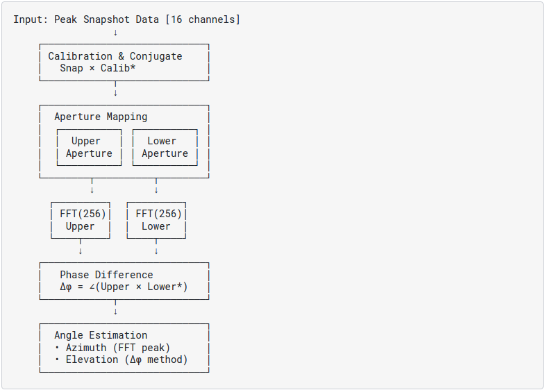
The processing stages are described in detail below.
MIMO Snapshot Extraction & Calibration
Extracts 16 complex values from the Range-Doppler map at the detected peak.
Applies phase/amplitude calibration to compensate for hardware variations.
The Snap contains the virtual antenna array response for this target.
Aperture Mapping and FFT Processing
Separates the 16-channel snapshot into two vertical apertures.
Maps the snapshot data to the virtual apertures.
Performs Radix-4 FFT on both apertures.
Phase Difference Estimation
Complex Representation
Let the FFT outputs at the detected azimuth angle index
mibe:(6)#\[\begin{split}\text{AFFT_Upper}(mi) &= A_u \cdot e^{j\phi_u} \\ \text{AFFT_Lower}(mi) &= A_l \cdot e^{j\phi_l}\end{split}\]Where:
\(A_u, A_l\) - Magnitudes of upper and lower aperture responses
\(\phi_u, \phi_l\) - Phases of upper and lower aperture responses
Cross-Correlation Operation
(7)#\[\begin{split}\text{AFFT_Upper}(mi) \times \text{AFFT_Lower}^*(mi) &= \left[A_u \cdot e^{j\phi_u}\right] \times \left[A_l \cdot e^{j\phi_l}\right]^* \\ &= A_u \cdot e^{j\phi_u} \times A_l \cdot e^{-j\phi_l} \\ &= A_u \cdot A_l \cdot e^{j(\phi_u - \phi_l)}\end{split}\]Extract Phase Difference
(8)#\[\text{PhaseDiff} = \angle\left(A_u \cdot A_l \cdot e^{j(\phi_u - \phi_l)}\right) = \phi_u - \phi_l\]Note
This is the phase difference between the upper and lower apertures at the detected azimuth direction.
Angle Extraction
Azimuth Angle Estimation
The azimuth angle is extracted from the FFT bin index using a pre-computed lookup table.
Mathematical Relationship:
(9)#\[θ_{azimuth} = \arcsin\left(\frac{k \cdot λ}{N \cdot d}\right)\]where:
\(k\) - FFT bin index (relative to center)
\(N\) - number of FFT points
\(λ\) - wavelength
\(d\) - horizontal element spacing
In practice, the azimuth angle is obtained by:
azimuth = Aindex[mic_afft]
where
Aindexis a pre-computed lookup table andmic_afftis the FFT bin index with maximum magnitude.Elevation Angle Estimation
The elevation angle is calculated directly from the interferometric phase difference.
Mathematical Relationship:
(10)#\[θ_{elevation} = \arcsin\left(\frac{\text{PhaseDiff}}{2π \cdot d_{elevation}/λ}\right)\]where:
\(\text{PhaseDiff}\) - phase difference between upper and lower apertures (radians)
\(d_{elevation}\) - vertical element spacing
\(λ\) - wavelength
This relationship directly converts the measured phase difference into an elevation angle, exploiting the vertical separation between the upper and lower antenna apertures.
Range and Velocity calculation
Peak Position Interpolation
Refine range or doppler position beyond FFT bin resolution.
Use quadratic interpolation (parabolic fitting) on 3 adjacent bins.
Mathematical Model: Quadratic Interpolation
Parabola Fitting:
The parabola through three points is given by:
(11)#\[y = a(x - x_0)^2 + b(x - x_0) + c\]Peak Location Offset:
The peak location offset \(p\) is calculated as:
(12)#\[p = -\frac{b}{2a} = \frac{Y_{-1} - Y_{+1}}{2(2Y_0 - Y_{-1} - Y_{+1})}\]where:
\(Y_{-1}\) is the value at the previous bin
\(Y_0\) is the value at the current bin (peak)
\(Y_{+1}\) is the value at the next bin
Interpolated Position:
The interpolated range bin position is:
(13)#\[\boxed{x_{\text{range}} = x_0 + p}\]Note
This quadratic interpolation provides sub-bin accuracy, typically improving accuracy by a factor of 2-10 depending on SNR, with up to 10x or more improvement achievable in high-SNR conditions.
Frequency calculation
Fast-time Frequency (\(f_{\text{fast}}\))
Frequency in the range FFT domain
Related to the beat frequency from target reflection
Encodes: Range + Velocity contribution
Slow-time Frequency (\(f_{\text{slow}}\))
Frequency in the doppler FFT domain
From phase change between consecutive chirps
Encodes: Velocity + Range-doppler coupling
Velocity Calculation with Ambiguity Resolution a. Velocity equation
(14)#\[\boxed{v = f_{\text{fast}} \cdot C_{v,\text{fast}} - \left(f_{\text{slow}} + \frac{n}{T_{\text{PRI}}}\right) \cdot C_{v,\text{slow}}}\]Where:
\(n = (jj-3) \in \{-2, -1, 0, +1, +2\}\) = PRF aliasing index
\(jj \in \{1, 2, 3, 4, 5\}\) = Loop iteration index for testing velocity ambiguity hypotheses, where \(jj = 3\) is the baseline.
\(T_{\text{PRI}}\) = Pulse Repetition Interval (time between consecutive radar pulses, in seconds)
\(C_{v,\text{fast}}\) = Fast-time velocity coefficient
\(C_{v,\text{slow}}\) = Slow-time velocity coefficient
Why Ambiguity Resolution?
Problem: Due to doppler aliasing, the true velocity might be:
(15)#\[v_{\text{true}} = v_{\text{measured}} + n \cdot v_{\text{PRF}}\]Where \(v_{\text{PRF}} = \frac{\lambda}{2 T_{\text{PRI}}}\) is the unambiguous velocity.
Solution: The algorithm tests 5 hypotheses (\(n = -2, -1, 0, +1, +2\)) and selects the one within the physically expected velocity range.
Range Calculation
(16)#\[\boxed{R = (f_{\text{fast}} - f_{\text{slow}}) \cdot C_R}\]Where:
\(C_R\) - Range coefficient (defined below)
Range Coefficient:
(17)#\[C_R = \frac{c}{2} \cdot \frac{T_{\text{chirp}} \cdot T_{\text{PRI}}}{B \cdot T_{\text{PRI}} - \Delta f \cdot T_{\text{chirp}}}\]
Design Requirements#
The number of horizontal antenna apertures is fixed to 8.
The number of vertical antenna apertures is fixed to 2.
Implementation Details#
Dataflow Configuration#
Use 1 SQDF (SequenceDataflow) to transfer the calibration vectors and peak count.
Use 1 SQDF (SequenceDataflow) to transfer the peak indices.
Use 1 SQDF (SequenceDataflow) to transfer the peak snap data.
Use 1 GSDF (GatherScatterDataflow) to transfer the NCI final data.
Use 1 SQDF (SequenceDataflow) to transfer the output data (target parameters).
Input and output tiling#
The peak snap, indices and output target parameters data are tiled in order to fit into the VMEM and support any arbitrary number of peaks. The tile dimensions are calculated based on the maximum input tile size constraint and the data dimensions. The tiling constraints are:
The tile size is set to maximize the number of peaks per tile, which is 128. For the peak snap, the tile width is set to 16 x 2 = 32, and the tile height is set to 128. For the peak indices, the tile width is set to 128, and the tile height is set to 3. For the output target parameters, the tile width is set to 128, and the tile height is set to 7.
Antenna aperture processing#
This stage creates two virtual apertures from the physical RX channels to enable interferometric estimation. The PVA implementation takes advantage of PVA vlookup and vast instructions to achieve the synthetic aperture mapping. It first transposes peak snap data in group of 8 to the intermediate buffer, and then uses vlookup and vast instructions to map the peak snap data to the virtual aperture efficiently.
Phase difference estimation#
The kernel performs Radix-4 FFT to transform the peak snap data to spatial frequency domain for both upper and lower apertures. It then combines the magnitude for peak detection. For Phase difference calculation, it firstly multiplies upper FFT values with conjugate of low FFT values, and then uses Arctangent to extract the phase difference. There is no native instruction for Arctangent in VPU, so the kernel uses sampler APIs and DLUT to approximate the Arctangent of the phase difference. A 513-entry LUT provides a good balance between memory usage and approximation accuracy.
Angle estimation#
The angle estimation requires to be performed in two steps: 1. Azimuth angle estimation: The algorithm searches the maximum peak in the spatial frequency domain and uses the position index to get the azimuth angle from a pre-computed angle lookup table. 2. Elevation angle estimation: The algorithm calculates the elevation angle using the interferometric phase difference between two vertically separated apertures.
Peak position interpolation#
The kernel uses GSDF to transfer in a patch of NCI final data for a specific peak. To handle circular indexing in Doppler domain, DOA operator uses CmdMemcpy APIs to generate circular padding for NCI final data before submit the DOA command program. The step is handled internally in DOA operator, and hidden from user.
Performance#
The DOA operator is compute-bound and scales with the number of detected peaks. The time consumption can be decomposed into three parts:
The FFT processing, which is compute-bound and scales with the number of detected peaks.
The angle estimation, which is compute-bound and uses sampler APIs for phase difference and elevation angle calculation.
The peak position interpolation, which is compute-bound and uses GSDF to transfer 32 patches of NCI final data per transaction (one patch per peak). This batch transfer strategy enables efficient sub-bin processing in the inner compute loop.
The test cases for profiling uses 71 peaks and tile size is fixed to 128.
Execution Time is the average time required to execute the operator on a single VPU core.
Note that each PVA contains two VPU cores, which can operate in parallel to process two streams simultaneously, or reduce execution time by approximately half by splitting the workload between the two cores.
Total Power represents the average total power consumed by the module when the operator is executed concurrently on both VPU cores.
Idle power is approximately 7W when the PVA is not processing data.
For detailed information on interpreting the performance table below and understanding the benchmarking setup, see Performance Benchmark.
NumPeaks |
Execution Time |
Submit Latency |
Total Power |
|---|---|---|---|
71 |
0.285ms |
0.153ms |
10.436W |