RadarNCI (Non-Coherent Integration)

Overview

Non-Coherent Integration (NCI) [1] [2] is a fundamental radar signal processing technique used to improve signal-to-noise ratio (SNR) by combining multiple radar returns across Rx channels and Doppler dimensions. The algorithm performs power-based accumulation of range-Doppler maps, which is particularly effective when phase coherence cannot be maintained across all measurements. NCI is an important step in automotive radar applications where it enables robust target detection in noisy environments by leveraging diversity from multiple Rx antennas and multiple Doppler measurements.

Algorithm Description

The NCI implementation uses the following processing scheme:

1. The NCI processing input consists of:

   1. FT2D, 2D FFT output representing the range-Doppler map with complex values for each RX antenna

2. The algorithm produces three outputs:

   1. nciRx, unfolded range-Doppler map representing the NCI combined data over RX antennas

   2. nciFinal, folded range-Doppler map accumulated over Doppler folds

   3. noiseEstimate, estimated noise level computed per range bin, can be disabled optionally

3. The processing flow is as follows:

   for each tile in the input data:
      // Stage 1: Accumulate power across RX channels
      for each pair of RX channels:
         nciRx += |FT2D[rx]|² + |FT2D[rx+1]|²
   
      // Average across RX channels
      nciRx = nciRx >> log2(numRxChannels)
   
      // Once all Doppler bins are accumulated, accumulate across Doppler folds
      // Stage 2: Accumulate across Doppler folds
      for each group of 4 Doppler folds:
         nciFinal += sum of 4 consecutive Doppler fold segments from nciRx
   
      // Average across Doppler folds
      nciFinal = nciFinal >> log2(numDopplerFolds)
   
      // Stage 3: Compute noise estimate
      noiseEstimate = min_nciFinal * threshold
   

Notes:

1. The Rx channels are processed in pairs and the Doppler folds are processed in groups of 4. This is done to keep these values configurable. If the NCI algorithm fixes the number of Rx channels and the number of Doppler folds, then the algorithm can be optimized for the specific values by removing the pair and group processing and doing away with a lot of the conditional logic.

2. The noise estimation is performed along with the NCI computation.

3. Input tiles may not have all Doppler bins for a channel, so the NCI accumulation for Doppler folds and noise estimation are done after all Doppler bins are accumulated, which may be after one or more input tiles are processed.

Design Requirements

1. The number of Doppler samples divided by the repeat fold must be at least 16, and the total samples must be divisible by 8.

2. The number of range bins must be a multiple of the tile height.

3. The combination of number of range bins, RX channels and number of samples must not exceed the tile dimensions.

4. The number of RX channels is limited to 2, 4, 8, 16, 32 and 64.

5. The combination of number of range bins, RX channels and number of doppler bins must not exceed the tile dimensions.

6. The number of doppler bins must be divisible by 8.

7. There should be at least 4 Doppler folds, and the number of Doppler folds must be a power of 2.

8. There should be at least 32 doppler bins in a Doppler fold, and the number of doppler bins in a Doppler fold must be divisible by 32.

9. The number of Doppler bins should be a multiple of the number of RX channels.

Implementation Details

Input Tiling

The tile dimensions are calculated based on the maximum input tile size constraint and the data dimensions. The tiling constraints are:

• The tile width is set to maximize the number of samples per tile

• Each tile fits within the VMEM constraints

NCI Accumulation

The NCI accumulation is performed in multiple stages:

Stage 1 - RX Channel Integration: The algorithm processes RX channels in pairs as the number of RX channels is configurable and even. For each pair, it computes the power (magnitude squared) and accumulates across all RX channels. The first pair initializes the accumulation buffer, while subsequent pairs add to it. After all channels are accumulated, the result is averaged by right-shifting by log2(numRxChannels).

Stage 2 - Doppler Fold Accumulation: The unfolded Doppler data is reorganized into folded segments. Groups of 4 Doppler folds are processed together using SIMD operations. This is done to keep the number of Doppler folds configurable. The accumulation across folds improves SNR for targets with ambiguous Doppler. The final result is averaged by right-shifting by log2(numDopplerFolds).

Stage 3 - Noise Estimation: Concurrent with the NCI processing, noise statistics are computed for each range bin. This provides a reference for subsequent detection algorithms. The agen minmax collection is used to get the minimum values of the NCI accumulation buffer per range bin, which is then used to estimate the noise level by scaling it by a threshold.

The overall device-side processing flow is illustrated in the following figure:

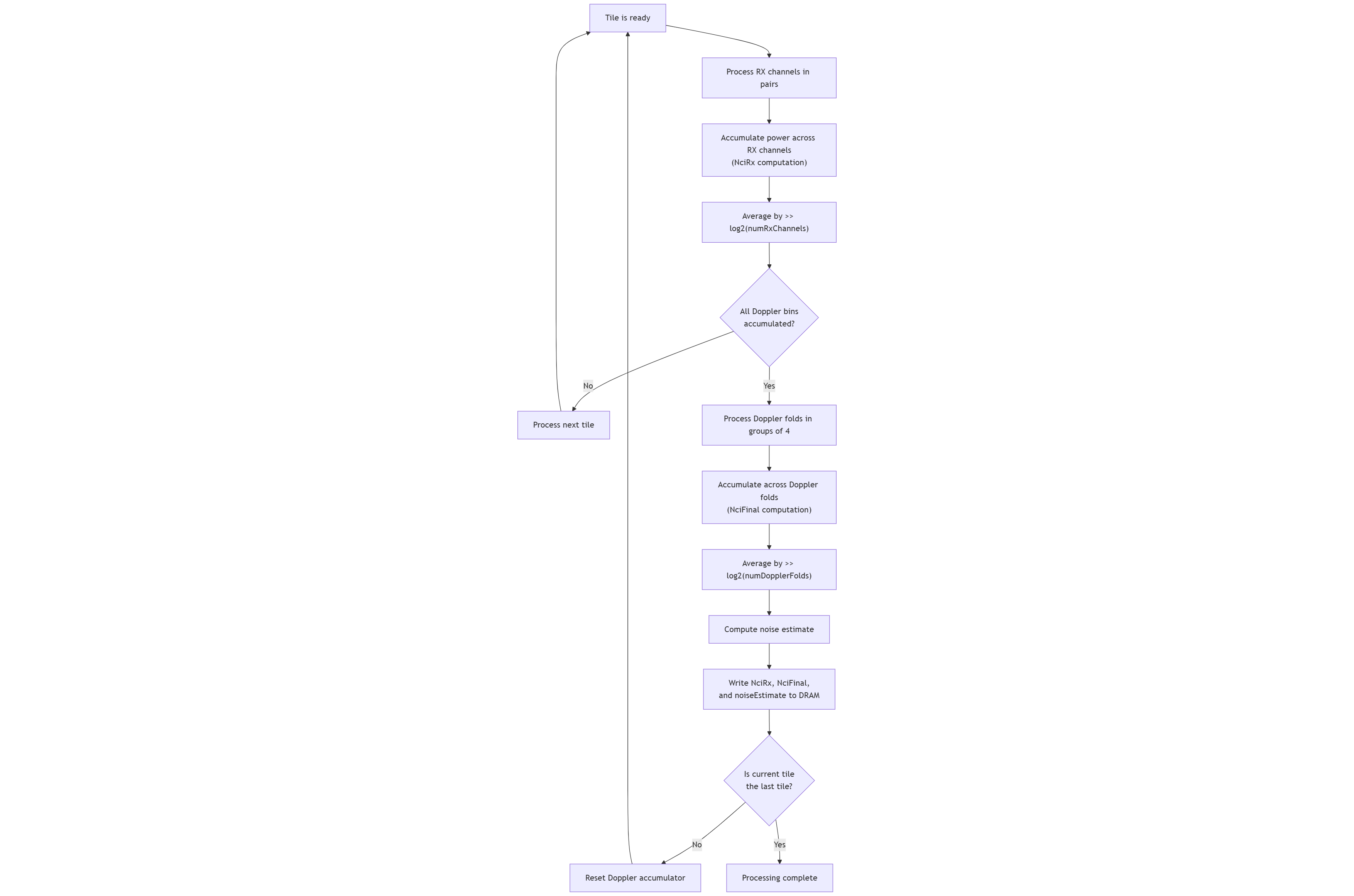
Figure 1: NCI’s Device Side Processing Flow

Performance

The NCI algorithm’s performance characteristics can be decomposed as follows:

1. The NciRx kernel is compute-bound and scales with the tile dimensions.

2. The NciFinal kernel is memory bound.

3. The noise estimation adds minimal overhead as it operates along with the NciFinal processing.

The implementation is optimized for typical automotive radar configurations with:

• 2-8 RX channels

• 512 or 1024 Doppler bins (64 or 128 folded bins)

• Range dimensions that are multiples of the tile height

Execution Time is the average time required to execute the operator on a single VPU core. Note that each PVA contains two VPU cores, which can operate in parallel to process two streams simultaneously, or reduce execution time by approximately half by splitting the workload between the two cores.

Total Power represents the average total power consumed by the module when the operator is executed concurrently on both VPU cores. Idle power is approximately 7W when the PVA is not processing data.

For detailed information on interpreting the performance table below and understanding the benchmarking setup, see Performance Benchmark.

RangeBinCount	RxAntennaCount	DopplerBinCount	DopplerFolds	Execution Time	Submit Latency	Total Power
128	2	512	4	0.078ms	0.021ms	13.346W
128	2	512	8	0.082ms	0.020ms	13.346W
128	2	512	16	0.090ms	0.020ms	13.245W
128	2	1024	4	0.137ms	0.021ms	14.517W
128	2	1024	8	0.142ms	0.021ms	14.416W
128	2	1024	16	0.151ms	0.020ms	14.315W
128	4	512	4	0.136ms	0.020ms	14.416W
128	4	512	8	0.140ms	0.020ms	14.315W
128	4	512	16	0.151ms	0.020ms	13.83W
128	4	1024	4	0.262ms	0.022ms	15.102W
128	4	1024	8	0.273ms	0.022ms	15.002W
128	4	1024	16	0.297ms	0.021ms	14.517W
128	8	512	4	0.271ms	0.021ms	14.517W
128	8	512	8	0.282ms	0.020ms	14.517W
128	8	512	16	0.307ms	0.020ms	14.416W
128	8	1024	4	0.505ms	0.022ms	15.101W
128	8	1024	8	0.516ms	0.022ms	15.101W
128	8	1024	16	0.540ms	0.021ms	14.618W
256	2	512	4	0.140ms	0.021ms	14.517W
256	2	512	8	0.146ms	0.021ms	14.416W
256	2	512	16	0.162ms	0.020ms	13.931W
256	2	1024	4	0.257ms	0.025ms	15.302W
256	2	1024	8	0.266ms	0.027ms	15.201W
256	2	1024	16	0.285ms	0.026ms	15.002W
256	4	512	4	0.255ms	0.022ms	15.101W
256	4	512	8	0.264ms	0.021ms	14.618W
256	4	512	16	0.285ms	0.021ms	14.517W
256	4	1024	4	0.508ms	0.026ms	15.686W
256	4	1024	8	0.531ms	0.024ms	15.201W
256	4	1024	16	0.577ms	0.026ms	15.001W
256	8	512	4	0.526ms	0.022ms	15.101W
256	8	512	8	0.549ms	0.021ms	15.002W
256	8	512	16	0.597ms	0.021ms	14.517W
256	8	1024	4	0.994ms	0.026ms	15.686W
256	8	1024	8	1.017ms	0.026ms	15.596W
256	8	1024	16	1.064ms	0.026ms	15.212W

Reference

1. M. A. Richards, “Fundamentals of Radar Signal Processing”, 2nd Edition, McGraw-Hill, New York, 2014.

2. M. A. Richards, “Notes on Noncoherent Integration Gain”, Georgia Tech Research Institute, 2014.