

Validate Personalized Purchasing Patterns
Compare personalized recommendations with simple baselines to decide which customer groups should receive them and which need a fallback. Before launching a personalized product campaign, verify that its recommendations reflect useful customer preferences. Familiar products can look convincing even when recommending popular products would work just as well.
Data scientists and ML engineers can use Kumo Engine to build this review. Kumo Engine learns from connected customer, purchase, and product records to rank possible future purchases. Shared products can connect a customer’s history to purchases by other customers, providing related context to investigate.
Your application combines those predictions with baseline comparisons, dated source records, and available model diagnostics so the merchandiser can inspect and challenge the result.
The recorded synthetic example uses a prediction cutoff of 2024-12-01: Customer C (synthetic customer 661) has 9 purchases in the preceding 90 days, concentrated in kitchen. Product A (product 79, kitchen) leads the model’s list, while Product B (product 48, stationery) leads the popularity comparison. The review tests whether this reflects useful personalization across similar customers.
Run the worked example
Download the Snowflake notebook and its companion helpers.
Extract the archive, upload the notebook and personalized_purchasing_patterns directory together into Snowflake Workspaces, and follow Snowflake notebook setup to connect a GPU service.
Run all cells to generate the data, train, score later records, compare baselines, and open the notebook controls.
The notebook also writes an offline HTML review page and retains results on runtime-local storage; export those files before stopping compute.
Results from the synthetic benchmark
Demonstration only. The executed example uses 690 synthetic customers, the full 80-product catalog, and 1,380 customer/cutoff pairs across December 1, 2024 and January 1, 2025. Customers predominantly repurchase four favored products from one category.
Of those pairs, 1,207 have eligible future purchases and 173 have none. The model and baselines use the same cutoffs and outcomes; personal frequency uses the preceding 90 days.
The popularity backfill control fills short personal lists with popular products. The unfilled personal list averages 3.69 items; the other methods return five.
Kumo’s recall difference against that filled baseline is 0.169, with a paired 95% customer-bootstrap interval of 0.153 to 0.188. The run used Kumo Engine 1.0.1 with the FAST preset on Snowflake GPU compute.
The result changes with available history. For customers with no recorded interactions, recall is 0.092 for Kumo and 0.056 for popularity. Their difference is 0.036, with an interval of -0.067 to 0.132; this test does not show a clear advantage over popularity for that group.
The frozen-model replay changed scores slightly while leaving every reviewed top-five category share unchanged. Its selected and control masks overlap on 16 of 24 removed rows, limiting the contrast.
Inspect both strong and weak results. Do not treat sensitivity as a causal explanation or synthetic performance as a production estimate.
Define the purchase prediction
For a related training and scoring example using synthetic purchase histories, see Recommend products from synthetic purchase histories. That example does not reproduce the separate Snowflake benchmark above.
Use the following customer, product, and purchase schema.
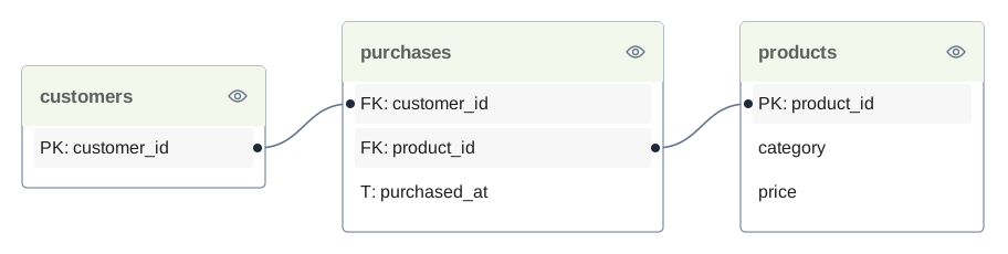
Keep source extracts that can reconstruct what was known at each prediction cutoff, including product attributes and campaign eligibility.
Use a predictive query, which specifies what to predict and over which time window, to rank products a customer may purchase during the next 30 days:
LIST_DISTINCT makes repeated purchases of a product one target product in that window.
The target includes both repeat and first purchases.
The returned ranking scores order products for a customer; they are not calibrated purchase probabilities. This temporal link prediction task estimates future observed purchases, not the additional purchases caused by showing a recommendation.
Train on earlier periods and evaluate on later periods with fully observed 30-day outcomes. Keep label windows within their chronological split boundaries and future purchases out of the input context.
Preserve customer IDs, prediction cutoffs, ranked products, and subsequent outcomes so comparisons refer to the same examples. See Predictive Queries for target and time-window semantics.
Turn a purchasing pattern into a test
State the hypothesis before inspecting test results: for customers with an established category preference, the personalized ranking retrieves future purchases better than a popularity ranking.
Define category preference from history available before each cutoff. For example, choose a history window and a minimum purchase count, then identify customers whose purchases are concentrated in one category.
Select these definitions using business requirements and validation data, and keep them fixed for the test period. Category concentration defines a group to investigate; it does not establish that the model uses category information.
Keep three questions separate:
- Does the pattern exist in the records? Measure category concentration, repeat purchases, and time since purchase from dated source rows.
- Does the recommender behave consistently with it? Compare recommended categories and future-purchase retrieval across customer groups, including customers with different preferences.
- Does personalization add predictive value? Compare with simple baselines on the same examples and outcomes.
Compare against simple alternatives
Build two baselines from purchases available before each prediction cutoff:
Choose the history window and tie-breaking rules on validation data. Apply the same cutoff-specific eligible catalog, customer population, and top-five limit to the model and baselines.
Record whether availability, campaign rules, or candidate truncation changed a list, and allow any method with insufficient eligible candidates to return fewer than five products. Keep purchase outcomes outside the eligible catalog visible as a separate coverage limitation.
Treat distinct eligible future purchases as binary relevance labels. Compare recall@5, the share of those products retrieved, and NDCG@5, which also rewards placing relevant products higher.
Report customer counts, target counts, and recommendation coverage alongside results for the overall population and each preference group. Use the same rule for customers with no future target products, and report their count separately rather than silently dropping them. Inspect the spread of results across customers and time periods before treating a small average difference as a reason to change the campaign.
Better retrieval in the relevant groups supports using personalization for that prediction task. Lists that differ across customers establish variation; the baseline comparison establishes whether that variation helps predict observed purchases.
Investigate one customer’s recommendation
Choose a mapped held-out example for Customer C using information available at its cutoff. Include examples where the model loses to a baseline as well as examples where it wins.
Product A is the model’s highest-ranked eligible product. Choose Product B as the highest-ranked different product from the popularity baseline, without looking at later purchases.
Show both products in one evidence view:
- Ranking difference: the model rank and raw score where returned, plus each product’s popularity rank.
- Recorded difference: category, price, prior purchase count, and most recent purchase, linked to source rows available before the cutoff.
- Outcome check: whether either product was purchased during the following 30 days, displayed separately from input history.
- Group result: the baseline comparison for customers with a similar history profile, including sample size and failures.
If Product B is absent from the returned model ranking, label its model rank and score as unavailable. Do not assign a zero score or infer that a business rule removed it.
Use available explanations to guide inspection:
Temporal link prediction supports eligible gradient and sampled-graph diagnostics, but not native column-cohort analysis. Check artifact availability and require a clear mapping from the sample to Customer C and its cutoff. Reading retained training artifacts does not generate explanations for arbitrary new predictions.
Keep model-wide findings separate from Customer C’s evidence. Unsigned sensitivity does not show whether a feature raised a product’s score, and shared sampled-graph importance does not decompose the score difference between A and B. Missing scores remain unavailable.
For diagnostic eligibility and artifact access, see Model Explainability.
Put the evidence in the merchandiser’s workflow
Lead the review card with a decision and keep the supporting records expandable. For the worked example, organize the review around three operator questions:
What needs review? Customer C’s personalized list differs from the popular-product list. Decide whether customers with this history profile should receive personalized recommendations.
What supports the recommendation? Product A matches Customer C’s historical category preference. Compare its dated purchase records with Product B, then inspect the group’s future-purchase retrieval against both baselines.
What should we do next? Use the group evaluation to choose the recommendation method. Investigate failures or stale records before expanding the campaign.
Show the cutoff, product comparison, group metrics, and available diagnostics under that summary. Allow the merchandiser to flag a poor recommendation, inspect a source record, or request a different comparison. Keep campaign permission, stock, and product eligibility checks owned by their authoritative systems.
Extend the review to sparse histories
Repeat the evaluation for customers with no recorded purchases, limited history, and established history. Define the groups using only information available at each cutoff. Separate customers unseen during training who already have purchase history from customers with zero interactions.
Test whether each group can be scored and whether its recommendations are useful before promising a fallback or personalized experience. New products are another case: verify candidate eligibility and scoring support separately from new-customer behavior.
Where a group does not improve on the selected baseline, consider using that baseline and measure the resulting coverage. Use the sparse-history analysis to guide deployment rather than relying on a single convincing example.
Build and verify the review workbench
Start with historical predictions, matched outcomes, and an evidence view for mapped test examples. Verify cutoff alignment, catalog rules, and baseline construction before interpreting model importance. Test whether a merchandiser can identify an unsupported explanation and choose an appropriate next action.
For a stronger claim that the model responds to a purchasing pattern, add controlled replay against a frozen model. Use plausible changes to the available history, such as removing a selected recent purchase, while preserving relationship integrity, the cutoff, and comparable sampling conditions. Compare the response with matched random or low-influence changes; retraining comparisons can test the predictive value of an entire information source.
These experiments test model behavior. Measure the effect of showing recommendations on sales or other business outcomes through an appropriate production experiment.
To apply the reviewed rankings to a campaign, continue with Personalized Email Recommendations.