

Review a credit default prediction
An analyst opens Account 17868 because its estimated probability of default is 56.4%, above the review cutoff of 50%. The account subsequently defaulted in October. That outcome tells us the flag was correct in this case. To understand the prediction, start with the six statements available when the model scored it.
This worked example uses a research credit-review prototype built around Kumo Engine output. Its account selector, field panels, and review workflow are application features. The displayed probability comes from the model’s calibrated output. The relevant-walk method requires a compatible Engine source build; it is separate from the released Model Explainability artifacts.
Start with the records
Account 17868 connects to statements from April through September 2005. September’s statement, record 107213, records a repayment status of one month late, a bill of NT$190,105, and a previous payment of NT$0. These are recorded inputs, before any explanation is computed.
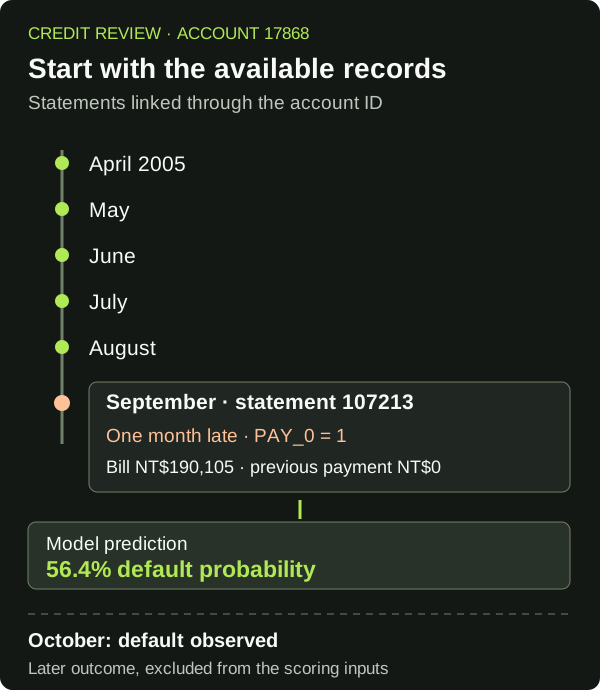
First confirm the account, statement identifiers, and information cutoff against the source records. Then distinguish three questions:
- Was the statement available to the model at the prediction cutoff?
- How did its encoded information contribute to the score?
- How would a small numerical input change affect that score?
A linked statement establishes context; it does not by itself establish contribution or direction.
Follow September through two updates
The local graph places September alongside the other five statements linked to Account 17868. Before following a route, distinguish the source record from its encoding: the model transforms the statement’s columns into a numerical vector that also carries representation components such as timing. The side-by-side view highlights that one vector inside the sampled context.
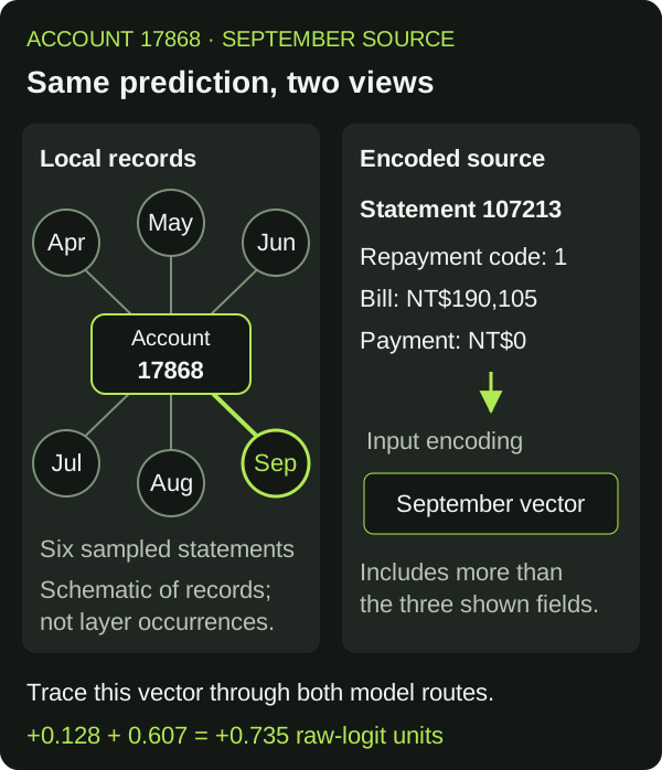
The model updates the representations of accounts and statements in two message-passing rounds. September’s information can reach the final account representation by two routes:
- Send it to the account in the first round, then update the account again.
- Update the statement in the first round, then send that updated information to the account.
The stored walk attribution assigns +0.128 to the first route and +0.607 to the second, rounded to three decimals. Together they account for +0.735 raw-logit units for September’s encoded source. Both signs point toward a higher raw default score.
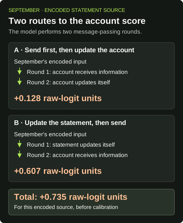
For this account, the route through September’s first-round statement update received the larger allocation: +0.607 versus +0.128. The analyst can now check the late-payment code and zero previous payment against the recorded statement, then ask a model reviewer to inspect how that update used September’s encoded information. This connects a source record to a particular learned calculation, rather than stopping at a ranking that says September mattered. It does not show that changing the update order would improve the prediction. The routes are paths through the learned computation, rather than additional financial transactions. See Relevance scores and graph walks for the redistribution rule and compatibility requirements.
Reconcile the units before interpreting the fields
The route values explain an uncalibrated raw logit, rather than percentage points of default probability. The model calibrates the final raw score before the prototype displays 56.4%. Positive source contributions can exceed the final raw score because other contributions are negative. Bias terms, statement timing, and numerical residuals also belong in the accounting.
September’s encoded-source allocation includes more than the three fields visible in the prototype’s monthly panel. Do not expect a sum of those visible field allocations to equal +0.735. Likewise, a field’s relevance and its gradient answer different questions: relevance allocates score to the recorded value; a gradient measures local numerical sensitivity. The prototype’s signed field gradients for this binary prediction are application research calculations, separate from Engine’s regression-only numerical sensitivity path. For a discrete repayment code, test another allowed value by rescoring rather than treating the local slope as a guaranteed effect of a whole-code change. Continue with Gradients and local subgraphs.
Decide what the review establishes
Tie the explanation to the saved prediction, model checkpoint, and sampled graph before comparing cases. Check that all score components reconcile and evaluate the explanation on additional known cases, including incorrect flags and missed defaults. Accounting agreement checks the allocation; removal tests and other controlled comparisons examine whether it describes the model’s behavior faithfully.
This case supports a bounded statement: September’s recorded information received positive relevance along two model routes for a correctly flagged account. It does not establish that the statement caused default, that the probability is calibrated for another population, or that the explanation is sufficient for a credit decision. Use the Explainability overview to define the evidence your domain reviewer needs before selecting a model architecture.
Appendix: training and review assumptions
This example uses the Taiwan credit-card default dataset, accessed through PaMIR 0.4.0 and reshaped into accounts and monthly statements. The retained run configuration and case output establish the following conditions. These are conditions for interpreting this example, rather than a recommended credit-model training recipe.
Treat predictive quality, probability calibration for the intended population, and the explanation’s usefulness to a domain reviewer as separate evaluations. The held-out Engine ROC-AUC for this run is 0.774; a gradient-boosting baseline on the same account split scores 0.784. The walkthrough demonstrates traceability through a GNN, rather than an accuracy advantage over that baseline.