

Relevance scores and graph walks
Suppose two related records connect the same source information to an account being scored. Which connection did the model use, and did both connections support the score? A single ranking of source records cannot show that distinction. A relevant walk follows one ordered route through the GNN’s calculation and assigns it a signed share of a selected output.
The method comes from Schnake et al., Higher-Order Explanations of Graph Neural Networks via Relevant Walks, version 3. Its GNN-LRP algorithm applies layer-wise relevance propagation, which redistributes a model output backward through its layers. The Engine adaptation described here requires a compatible source build and the CPU model profile listed below; it is separate from released training explanation files.
Follow one record through two routes
Start with the fictional related tables below.
Two signals, A and X, connect to context records B and D, which connect to account C.
Signals A and X are rows, rather than individual columns within a row.
A signal has two foreign-key columns, context_1 and context_2, shown as FK1 and FK2 in the figure.
A primary key (PK) identifies a row; a foreign key (FK) points to a row in another table.
As in an Engine table relationship view, foreign keys describe how the tables connect.
For one prediction, Engine samples a bounded graph of individual records around the account.
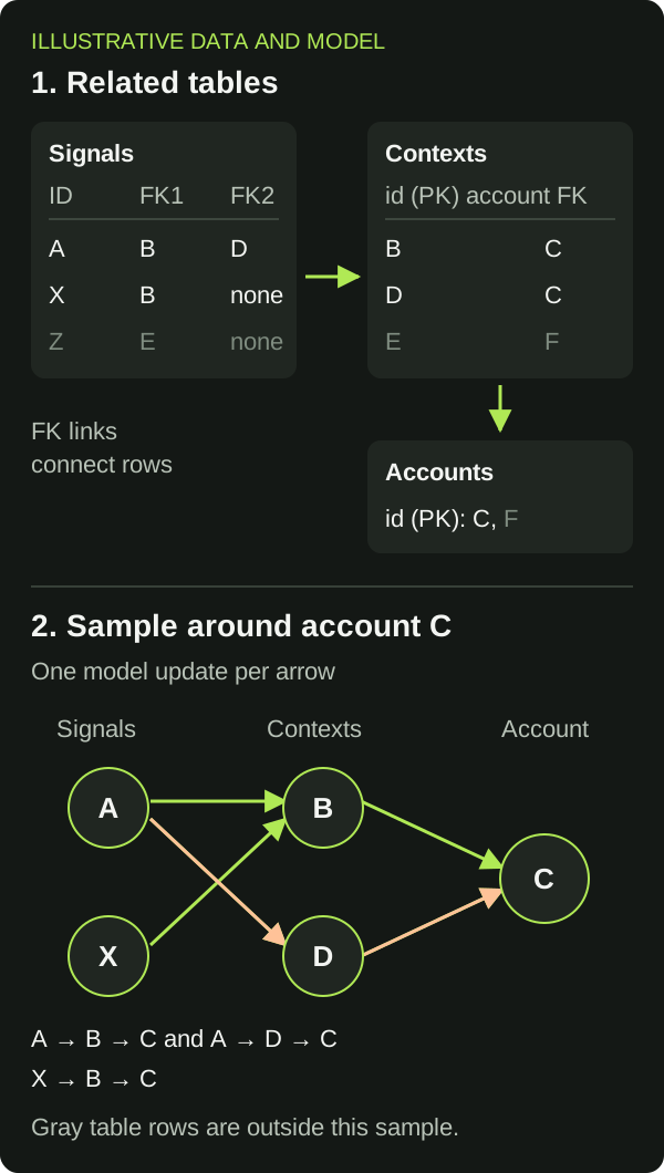
Assume a two-layer GNN produces an encoded regression output of 20 units for C. This is a teaching example with no bias or numerical remainder, rather than a measured Engine result. The attribution algorithm assigns the three routes these values:
A’s aggregate relevance is +10, but reporting only that total hides its opposing routes. The routes can have different signs because the model applies different learned weights and intermediate computations along them. A useful follow-up is to inspect why A’s information is used differently through B and D.
Each arrow in this example corresponds to one message-passing layer. In a general GNN, a walk can also include a self update, where a record carries its own information into the next layer. That computational step does not create a new relationship in the source tables.
To calculate the values, the GNN-LRP algorithm starts at C’s chosen output and redistributes relevance backward through the prediction head, the final layers that produce the selected output. At each layer, it allocates shares among incoming messages, self updates, and bias terms using the selected redistribution rule. It follows each share back to the source record’s encoded features, the numerical representation produced from the record’s columns. The +14 and −4 values are allocations along A’s complete routes, rather than measurements made by deleting either route.
Name the output before interpreting a sign
The selected output determines both the meaning of the sign and the units. Identify the task and output before comparing relevance values:
For binary classification, Engine checks the selected label against the fitted target encoder, which maps class labels to the model’s output. The probability shown to a reviewer can include a calibration step outside the explained raw logit. Transforming each relevance value with a sigmoid does not turn it into additive probability contributions.
Relevance also does not predict the effect of increasing A’s input or deleting A’s record. Use gradients and local subgraphs to distinguish local sensitivity from an allocation of the current score.
Reconcile the complete ledger
An interface may display only the routes selected for review. Suppose it shows A’s two routes and hides X’s computed route. The visible total is +10, while the model output remains +20. The ledger explains the difference:
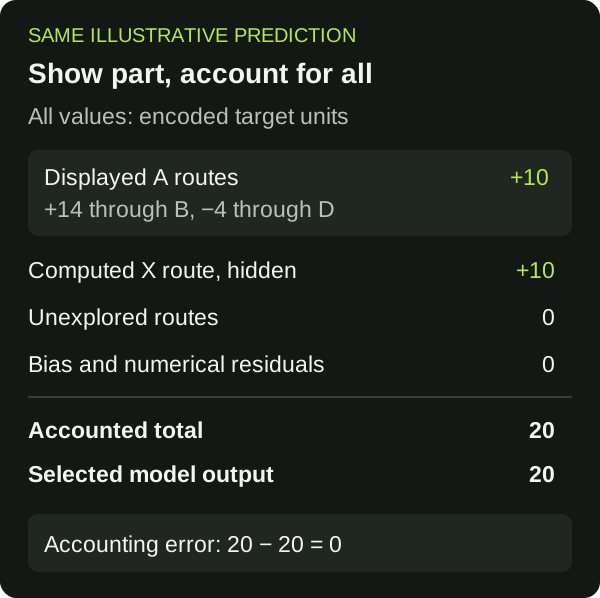
Accounting error means the selected output minus the total of all accounted terms. It is zero here because displayed routes (+10) and the hidden route (+10) already sum to the output (+20). It is not a prediction error against an observed target.
Real results can include additional terms:
- Omitted displayed walks were computed but hidden by the display limit, as with X’s route here.
- Omitted search mass reached routes the search did not finish exploring. This is different from hiding already computed walks.
- Bias relevance allocates score to learned additive offsets, rather than to a source route.
- Stabilizer and precision residuals account for numerical adjustments and differences introduced by the computation.
Read these terms and the search completion status before interpreting the largest displayed routes.
Positive and negative omitted values can cancel, so a small net remainder does not establish that all omitted records are unimportant.
Likewise, large opposing intermediate values can make numerical reconciliation less informative even when its error is small.
The denominator diagnostics report when positive and negative terms nearly cancel in the totals used for division.
If head_output_flipped is flagged, the output redistribution has reversed directional signs; do not interpret that row’s signs as straightforward support or opposition.
Choose and evaluate the attribution rule
Suppose you want to compare how A’s information travels through B and D. You need a consistent rule for dividing relevance whenever a layer combines several inputs. The method name records which rule produced the route values.
GNN-LRP supplies this backward allocation for compatible models, including models with learned bias offsets.
The paper-style weight-gamma rule can give extra weight to positive learned connections during redistribution; its gamma setting controls that emphasis.
An alternative contribution-gamma rule instead adjusts positive weighted input contributions.
When the inputs at every redistribution step are nonnegative, the two rules agree; they can differ on signed inputs.
Use the same rule and settings when comparing cases, and retain the method name with the result.
Degree-T GNN-GI is an optional research check when the question is whether complete walks form the exact mathematical decomposition described by the paper. Here, T is the number of message-passing layers, so the example has T = 2. A gate is a numerical multiplier on a connection at one layer. The algorithm varies these gates and uses nested Gradient × Input to calculate how their joint interaction contributes to the output. It requires a bias-free model and further checks on complete enumeration (checking every route), activation boundaries, and numerical precision before claiming an exact degree-T decomposition. It is not the required route for explaining an ordinary model with biases; use GNN-LRP for that profile. An exact claim concerns the captured computation with encoded inputs and fixed aggregation denominators, not raw feature contributions or the result of deleting records.
An attribution that adds up has passed an accounting check. To evaluate whether it identifies the model’s important evidence, use known examples, controlled removals or replacements, and comparison methods. Changing records can create unusual inputs or alter several routes together, so interpret those tests alongside their assumptions. Predictive accuracy, numerical reconciliation, and explanation faithfulness answer separate questions.
Check model compatibility before training
The Engine relevant-walk path requires:
- An evaluation-mode
HeteroGNNwith aNodePredHead. - ReLU or identity activations, no normalization, and one sum or mean aggregation.
- Registered relation and root operators, without prediction-time encodings, a distribution head, or a
torch.compilewrapper. - Scalar MSE regression, or binary node classification with binary cross-entropy and exactly two fitted target labels.
- CPU capture with one scorer and one seed per batch (
batch_size=1,num_workers=1).
Supported linear layers, self updates, and evaluation-mode dropout do not make unsupported operations compatible. GELU, LayerNorm, multiple aggregations, multiclass and multilabel tasks, link prediction, and forecasting are outside this walk profile. GPU and concurrent scoring are not qualified. For binary walks, numerical sensitivity must be disabled because that separate path supports scalar regression. An unsupported or failed attribution is a missing explanation, even when prediction succeeds.
Use the explainability overview to choose the evidence your reviewer needs before selecting a model architecture.