

Gradients and local subgraphs
A gradient asks how a small change in an input would affect a chosen model output near the current example. If the derivative is −0.4 output units per transformed input unit, increasing that input by 0.1 gives an approximate output change of −0.04, while other inputs and the sampled graph remain fixed. The approximation is local: a larger change can cross an activation boundary and behave differently.
Choose the diagnostic that answers your question:
Read a column ranking
Suppose you want to know whether the model is more sensitive to statement bill amounts or to previous payments across its explanation examples. A cell is one value at the intersection of a source row and column, such as one statement’s bill amount. A column ranking combines measurements from many records and examples into one score for each table column. It does not retain a separate signed contribution for each statement.
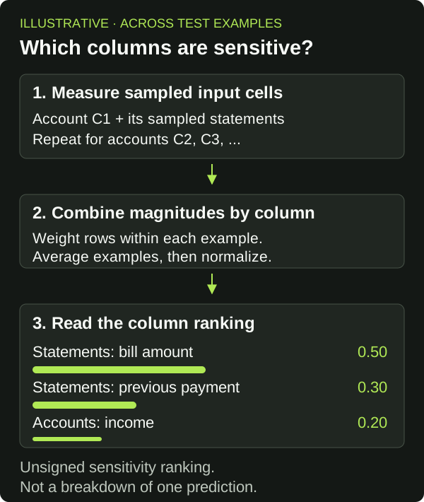
The figure shows the aggregation steps; its ranking values are illustrative, rather than results from a trained model.
The training gradient explainer computes input-column sensitivity while the selected model runs in inference mode. For binary classification it differentiates the positive-class logit; for multiclass classification it selects the largest class logit for each example. Other supported tasks use the raw logits or scores, including a sum across labels where applicable. This is a different output choice from explaining a calibrated probability or a decoded regression value.
An encoder converts source-column values into the numerical representations used by the model. The encoder exposes gradient magnitudes (absolute values) for each reported column in the sampled rows. Within an example, Engine combines row-level magnitudes with a weighted sum that gives more weight to larger gradients. This lets a column rank highly even when only a few related records carry the signal. It then averages across examples and normalizes column scores by their total when positive.
Use the resulting ranking to investigate whether the model responds to plausible inputs or a potential leakage column. The normalized score is not an allocation of the prediction and does not preserve the gradient’s sign. A score of 0.2 does not mean the column caused 20% of a customer’s default risk. Compare columns within the same retained explanation, using its selected model and explanation population.
The Model Explainability guide shows how to retrieve the selected training experiment’s scores.csv, cohort files, and sampled subgraphs.
Retain those files separately from the published model bundle.
Inspect the records around an example
Now narrow the question to one account prediction: which statements were included, and which values had the largest measured sensitivity in that example? Each sampled record is a graph node. A local cell score ranks the gradient magnitude for one cell within that captured subgraph.
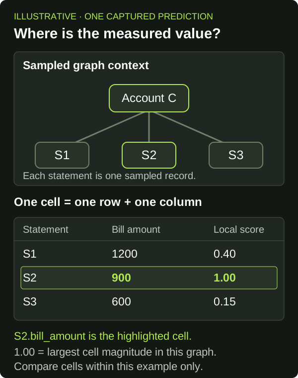
The values and scores in the figure are illustrative; bill amounts use arbitrary units. The table shows the bill amount cells, while the captured records can contain other columns. The highlighted 1.00 identifies the largest measured cell magnitude in this captured example; it is not a probability or a share of the prediction.
A sampled subgraph shows model context: selected records, relationships, feature values, and the prediction’s anchor time when recorded. It helps answer whether the expected monthly statements were reachable and sampled. Their presence establishes that the records were included in that captured context. It does not establish that each record had a nonzero effect on the output, or that the neighborhood is the full database graph.
Training artifacts cover a bounded selection of test examples. They are not the original scoring graphs for every future prediction. In the experimental batch explanation path, replayed context is also distinct from evidence captured during the original scoring forward pass. Keep the capture origin and prediction identity with the graph you inspect.
To produce these local cell scores, Engine takes the absolute gradient magnitudes and divides them by the largest cell magnitude within that example. The largest cell therefore scores 1 when a nonzero measurement is available. These scores help compare cells within that graph; they do not express raw derivatives or additive contributions. The collector can combine rows beyond its display limit into an aggregate entry, so inspect whether a node represents one source record or a group.
Measure sensitivity during scoring
Original-pass numerical sensitivity belongs to the experimental Engine path. It is separate from the training diagnostics above and requires CPU scalar MSE regression with a numerical target encoder, one scorer, and one seed per batch. It does not provide this sensitivity measurement for binary classification or recommendation scores.
This path differentiates the emitted, decoded regression prediction with respect to the transformed numerical value entering the learnable encoder. That input has already undergone fitted imputation, scaling, optional logarithmic transformation, and clipping. Its units are therefore decoded output units per transformed input unit. They are not output units per raw dollar, item, or day.
The retained cell includes the transformed value, transformation settings, absolute gradient, and signed gradient when available. The sign describes a local increase or decrease in the selected decoded output. The magnitude describes sensitivity, not relevance allocated from the score. It does not establish the real-world consequence of changing a customer’s history.
The recorded raw value is the numerical tensor mapper’s input to the fixed transformation, at model input precision. Join retained source primary keys back to the original data when exact source values matter. An imputed value can have a valid gradient in transformed coordinates even though the original observation was missing. Read the missing-value and transformation fields together.
Distinguish zero from unavailable
A successfully calculated zero gradient means no local sensitivity was measured at that point in the chosen coordinates.
It can reflect an inactive computation or a locally flat function; it does not prove the input is irrelevant everywhere.
The original-pass artifact marks a row whose computed numerical gradients are all zero as zero_signal.
A missing measurement has a different interpretation. No sampled numerical inputs, disconnected inputs, absent source mappings, unsupported configurations, and capture failures are recorded separately. Do not replace these states with zero when building a chart or averaging results. Check row and cell statuses, the recorded reason, and manifest completion before comparing examples. Prediction output can remain usable while its diagnostics are incomplete.
When you need to allocate an output across computational routes, continue to relevance scores and graph walks. Use the overview to decide which evidence belongs in your review process.