Generating Embeddings for Protein Clustering#

In this example we will use the BioNeMo Framework to show how to

Load and work with data
Load a pretrained model
Extract embeddings
Build simple vizualisations
Perform a Clustering task with the embeddings

Prerequisites:#

Before diving in, ensure you have all necessary prerequisites. If this is your first time using BioNeMo, we recommend following the quickstart guide first.

Additionally, this tutorial depends on: - The ESM-1 model. - The local inference server.

Download the Pre-trained Models#

The basic building blocks are already implemented in the BioNeMo Framework. It comes with a set of scripts that make it easier to download pre-trained models from NVIDIA NGC.

As of the pre-release version (13 JUN 2023), we have the following models available:

Molecule/MegaMolBART
Protein/ESM-1nv
Protein/ProtT5nv

Once the container has been succesfully pulled and the .env file configured correctly, download the pre-trained models with

bash launch.sh download

The command above will invoke a routine that downloads the models from published addresses such as in /bionemo/ci/blossom/download_all_models.sh.

For example, we can see MegaMolBart being download from https://api.ngc.nvidia.com/v2/models/nvidia/clara/megamolbart_0_2/versions/0.2.0/zip.

Once execution is complete, you will see files with the .nemo extension within the folder specified in the DOCKER_MODELS_PATH configuration of your .env file.

Refer to the Quickstart Guide for more info about the .env file.

Run the container#

docker run -it -p 8888:8888 --gpus all -v <model directory>:<mount destination> <BioNeMo_Image> <model>

This example has been built upon a contaier running in a local machine with 2 x A6000 RTX GPUs. Refer to specific instructions for remote and multinode launch.

The comman above will set up a ‘Jupyter Lab’ that can be found on localhost:8888

.nemo Files
Make sure the models downloaded are within the desired project mount directory such as /models/protein/esm1nv; otherwise, you may have to move the .nemo files, such as esm1nv.nemo from wherever it has been downloaded into.

Jupyter Lab’s Workspace
If you type pwd in the Jupyter Lab’s terminal, this may not show BioNeMo’s original directory in your machine but yet another directory such as /workspace, according to the project mount directory you’ve set in the .env file.

In this example, we will be working with the ESM1-nv model, the UniRef50 and the UniProtKB Dataset by UniProt.org.

ESM-1nv was developed using the BioNeMo framework. The model uses an architecture called Bidirectional Encoder Representations from Transformers (BERT) and is based on the ESM-1 model

You may want to run the code as provided in the cells below - into a Jupyter Notebook launched from the JupyterLab interface running inside the container.

Download the data#

The Universal Protein Resource (UniProt) is a comprehensive resource for protein sequence and annotation data [1].

The UniRef is a set of Reference Clusters with sequences from the UniProt Knowledge base and selected UniParc records. UniRef50 is a “second derivation” of UniRef100: Uniref90 is generated by clustering UniRef100 seed sequences and UniRef50 is generated by clustering UniRef90 sequences. For more information, refer to the UniRef page.

Using BioNeMo features to download UniRef50#

The simplest and most reliable way to download the entire UniRef50 dataset is through the BioNeMo framework UniRef50Preprocess class which has the following features:

Runs a fasta indexer
Splits the data into train, validation and test sets
Writes the dataset in the appropriate directories within the BioNeMo Framework /tmp/uniref50/processed

For example,

from bionemo.data import UniRef50Preprocess
data = UniRef50Preprocess()
data.prepare_dataset()

In the snippet above,UniRef50 is downloaded. In the example below, we’ll pass the UniProtKB dataset as argument to the same function.

Alternative datasets#

We can also download datasets that are not available in the BioNeMo Framework. This can be done in two ways:

A) Using bash and wget pointing to the dataset’s URL

mkdir -p /tmp/data/protein/esm1nv  
wget -P /tmp/data/protein/esm1nv <URL>

B) Transfering from the local machine to the container

docker cp <dataset directory and filename> container_id:/<container directory and filename>

Generating Embeddings#

The BioNeMo-way is simple:

# Initalize the Inference Wrapper that will invoke the pre-trained model
esm = ESMInferenceWrapper()
# Work with a set of sequences (these are invalid sequences despite valid amino-acids)
sequence_examples = ["TRANSCENDINGLIMITS", "MASTERMINDING"]
# Generate Embeddings
embeddings = esm.seq_to_embedding(sequence_examples)

# Print the shape of embeddings
print(f"Shape of embeddings (2, 768): {embeddings.shape}")

This requires fewer lines of code than, for example, Rostlab’s Example in Hugging Face as the ESMInferenceWrapper class takes care of the tokenization process and the hidden states handling

Example#

Since we are now familiar with the basic building blocks of the BioNeMo Framework to generate Protein Embeddings, let’s tackle and example including data vizualization and clustering with the UniProtKB Dataset.

To perform this in an efficient manner, we will ustilize open-source CUDA accelarated data science and machiene learning libraries such as cuML, cuDF, cuPY. For more information, check out NVIDIA RAPIDS.

cuDF provides a pandas-like API that will be familiar to data engineers & data scientists, so they can use it to easily accelerate their workflows without going into the details of CUDA programming. Similarly, cuML enables data scientists, researchers, and software engineers to run traditional tabular ML tasks on GPUs. In most cases, cuML’s Python API matches the API from scikit-learn.

Note

The following cells containing python code snippets can be directly copied and executed into a Python environment such as a Jupyter notebook running in a BioNemo container.

%%time
import numpy as np              # numpy for simple array manipulations
import cudf                     # Using cudf from NVIDIA RAPIDS
import matplotlib.pyplot as plt # Matplotlib for data vizualization
import pandas as pd             # simple dataframe manipulation
import cuml                     # We will use DBSCAN for clustering with unkown labels and clusters
import cupy as cp               # To process arrays on the GPU
import torch                    # To deal with tensors


# bionemo utils
from bionemo.data import UniRef50Preprocess
from infer import ESMInferenceWrapper

# Dimensionality reduction algorithm 
from cuml.manifold import TSNE as cumlTSNE
from sklearn.preprocessing import StandardScaler

CPU times: user 79 µs, sys: 17 µs, total: 96 µs
Wall time: 98.2 µs

Internet Speed The step below downloads the UniProtKB Database with 569,516 entries. It can take a while to process depending on your internet connection speeds.

%%time
data = UniRef50Preprocess()     # Instantiate a new UniRef data process
'''
Downloads the UniProtKB Database 
The UniProtKB Dataset has 569,516 entries. 
'''
data.prepare_dataset(url="https://ftp.uniprot.org/pub/databases/uniprot/knowledgebase/complete/uniprot_sprot.fasta.gz",
                     num_csv_files=1,
                     val_size=85000,
                     test_size=85000)

[NeMo I 2023-07-10 10:50:09 preprocess:110] Data processing can take an hour or more depending on system resources.
[NeMo I 2023-07-10 10:50:09 preprocess:113] Downloading file from https://ftp.uniprot.org/pub/databases/uniprot/knowledgebase/complete/uniprot_sprot.fasta.gz...
[NeMo I 2023-07-10 10:50:09 preprocess:69] Downloading file to /tmp/uniref50/raw/uniprot_sprot.fasta.gz...
[NeMo I 2023-07-10 11:05:52 preprocess:83] Extracting file to /tmp/uniref50/raw/uniprot_sprot.fasta...
[NeMo I 2023-07-10 11:05:54 preprocess:221] UniRef50 data processing complete.
[NeMo I 2023-07-10 11:05:54 preprocess:223] Indexing UniRef50 dataset.
[NeMo I 2023-07-10 11:05:54 preprocess:230] Writing processed dataset files to /tmp/uniref50/processed...
[NeMo I 2023-07-10 11:05:54 preprocess:187] Creating train split...
[NeMo I 2023-07-10 11:05:58 preprocess:187] Creating val split...
[NeMo I 2023-07-10 11:05:59 preprocess:187] Creating test split...
CPU times: user 7.18 s, sys: 5.36 s, total: 12.5 s
Wall time: 15min 50s

%%time
'''
Breaks down the downloaded and processed files into 3 distinct sets
'''
train = cudf.read_csv("/tmp/uniref50/processed/train/x000.csv")
val = cudf.read_csv("/tmp/uniref50/processed/val/x000.csv")
test = cudf.read_csv("/tmp/uniref50/processed/test/x000.csv")

# Prints the length of the training set
print(f"Train set {len(train)} \
    \t Validation set {len(val)} \
    \t Test set {len(test)}")

Train set 399793     	 Validation set 85000     	 Test set 85000
CPU times: user 515 ms, sys: 41 ms, total: 556 ms
Wall time: 599 ms

Simplification In this example we will ignore val and test sets

train.head()

	record_id	record_name	sequence_length	sequence
0	349074	sp\|P29373\|RABP2_HUMAN	138	MPNFSGNWKIIRSENFEELLKVLGVNVMLRKIAVAAASKPAVEIKQ...
1	116060	sp\|A8A5E7\|EFG_ECOHS	704	MARTTPIARYRNIGISAHIDAGKTTTTERILFYTGVNHKIGEVHDG...
2	503050	sp\|Q72LF4\|TTUB_THET2	65	MRVVLRLPERKEVEVKGNRPLREVLEELGLNPETVVAVRGEELLTL...
3	356017	sp\|Q6D7Z7\|RECR_PECAS	201	MQTSPLLESLMEALRCLPGVGPRSAQRMAFQLLQRNRSGGMRLAQA...
4	343362	sp\|B0R808\|PYRD_HALS3	349	MYGLLKSALFGLPPETTHEITTSALRVAQRVGAHRAYAKQFTVTDP...

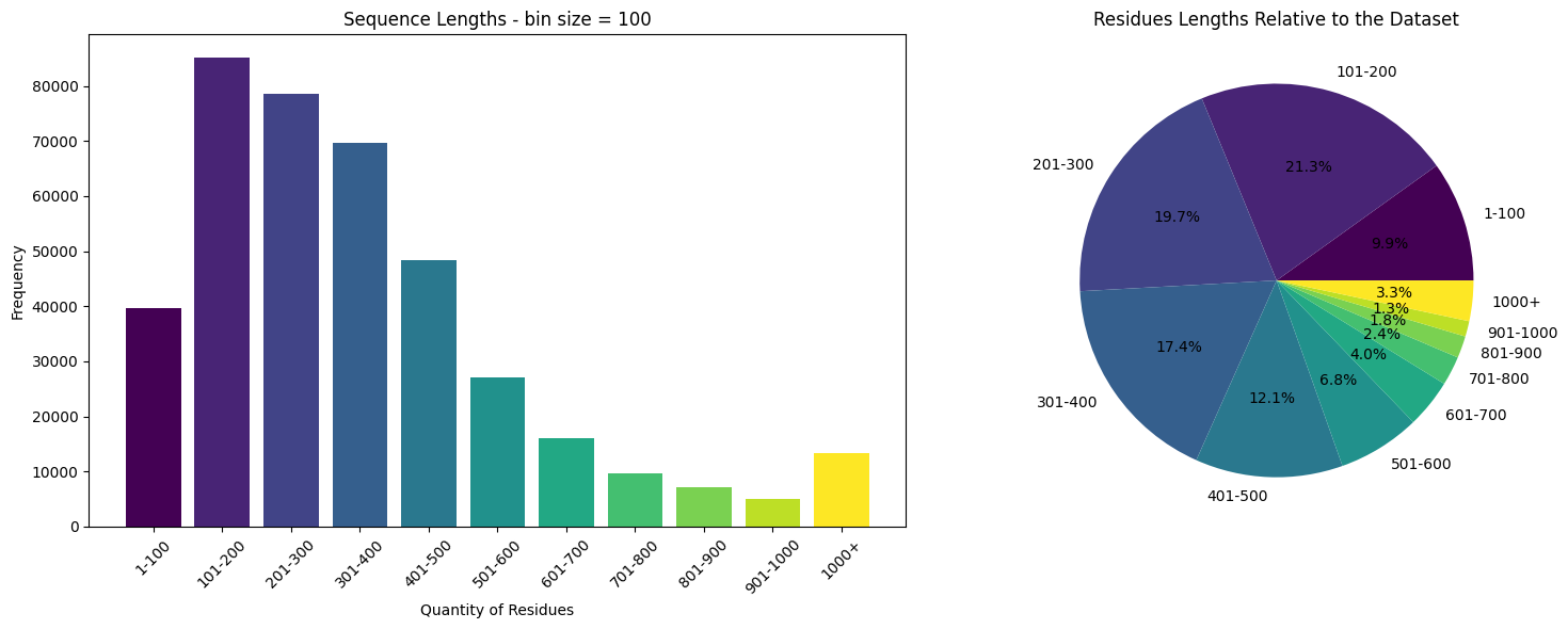
Let’s have a look on the train dataset

%%time
# Define the bin function
def bin_data(s, start, end, step):
    # Create the bins
    bins = list(range(start, end+1, step)) + [np.inf]

    # Create the labels
    labels = [f'{i+1}-{i+step}' for i in range(start, end, step)] + ['1000+']
    
    # Cut the Series
    s_cut = pd.cut(s, bins=bins, labels=labels, include_lowest=True, right=False)
    
    return s_cut

# we'll work with the sequences and their lengths
s = train.sequence_length.to_numpy()

# Bin the data
s_binned = bin_data(s, start=0, end=1000, step=100)

# Count the frequency of each bin
s_counts = s_binned.value_counts()

# Generate colors from the viridis colormap
colors = plt.cm.viridis(np.linspace(0, 1, len(s_counts)))

# Create a 1x2 grid of subplots
fig, axs = plt.subplots(1, 2, figsize=(16, 6))

# Create the bar plot on the first subplot
axs[0].bar(s_counts.index, s_counts.values, color=colors)
axs[0].set_title('Sequence Lengths - bin size = 100')
axs[0].set_xlabel('Quantity of Residues')
axs[0].set_ylabel('Frequency')
axs[0].tick_params(axis='x', rotation=45)

# Create the pie chart on the second subplot
axs[1].pie(s_counts.values, labels=s_counts.index, autopct='%1.1f%%', colors=colors)
axs[1].set_title('Residues Lengths Relative to the Dataset')

# Display the plots
plt.tight_layout()
plt.show()

../_images/9012fff04a1005d3e9ec7579a25050d9e1067e69e8b64018a2a40f87c5208388.png

CPU times: user 291 ms, sys: 223 ms, total: 515 ms
Wall time: 296 ms

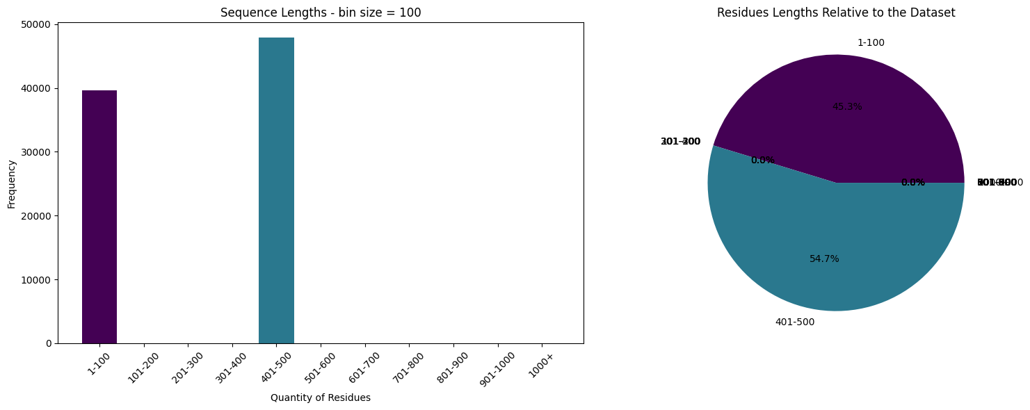
ESM-1nv limits#

The current limit for ESM-1nv is 512 Residues based on the nemo checkpoints, so we will have to decrease the dataset accordingly.

Data Cleaning#

We can also ignore the test and validation sets for this example (since we’re not training a model).

In this example, we will use two groups of proteins:

Up to 100 amino acids, which can include functional types such as

Regulatory Peptides: For example, Insulin, with 51 amino acids.
Neuropeptides: Small protein-like molecules used by neurons to communicate with each other. Substance P, a neuropeptide involved in pain perception, contains 11 amino acids.
Antimicrobial Peptides: These are an essential part of the innate immune response and have antibiotic properties. An example is defensins, which typically contain 18-45 amino acids.
Toxins: Many toxins produced by plants, animals, and bacteria are small peptides. For example, Melittin, the main toxin in bee venom, has 26 amino acids.
Cytokines: Some small cytokines, often referred to as chemokines, have less than 100 amino acids. An example is Interleukin-8 (IL-8), a chemokine produced by macrophages, with 99 amino acids.

Between 400 and 500 amino acids, with functional types
- G-Protein Coupled Receptors (GPCRs): This is a large family of proteins that span the cell membrane and receive signals from outside the cell. GPCRs are involved in a vast number of physiological processes and they typically have around 350-500 amino acids.
- Ion Channels: Ion channels are a class of proteins that allow ions to pass through the membrane in response to a signal. The length of these proteins varies, but many are within the 400-500 amino acid range.
- Cytochrome P450 Enzymes: These enzymes are involved in the metabolism of various molecules and chemicals within cells. They are typically around 400-500 amino acids long.
- Some Serine/Threonine Protein Kinases: This is a large family of enzymes that catalyze the addition of a phosphate group to serine or threonine residues in other proteins. While the length varies significantly, many members of this family are within the 400-500 amino acid range.
- Small GTPases: These are a family of hydrolase enzymes that can bind and hydrolyze guanosine triphosphate (GTP). The proteins are critical regulators of a wide variety of cellular processes. Many small GTPase proteins fall within the 400-500 amino acid range.

%%time
train = train[(train.sequence_length < 100) | ((train.sequence_length > 400) &  (train.sequence_length < 500))]
print("Max seq. lentgh (train)", train.sequence_length.max())
print("Length of dataset", len(train))

Max seq. lentgh (train) 499
Length of dataset 87517
CPU times: user 19.7 ms, sys: 0 ns, total: 19.7 ms
Wall time: 20.1 ms

%%time
# Define the bin function
def bin_data(s, start, end, step):
    # Create the bins
    bins = list(range(start, end+1, step)) + [np.inf]

    # Create the labels
    labels = [f'{i+1}-{i+step}' for i in range(start, end, step)] + ['1000+']
    
    # Cut the Series
    s_cut = pd.cut(s, bins=bins, labels=labels, include_lowest=True, right=False)
    
    return s_cut

# we'll work with the sequences and their lengths
s = train.sequence_length.to_numpy()

# Bin the data
s_binned = bin_data(s, start=0, end=1000, step=100)

# Count the frequency of each bin
s_counts = s_binned.value_counts()

# Generate colors from the viridis colormap
colors = plt.cm.viridis(np.linspace(0, 1, len(s_counts)))

# Create a 1x2 grid of subplots
fig, axs = plt.subplots(1, 2, figsize=(16, 6))

# Create the bar plot on the first subplot
axs[0].bar(s_counts.index, s_counts.values, color=colors)
axs[0].set_title('Sequence Lengths - bin size = 100')
axs[0].set_xlabel('Quantity of Residues')
axs[0].set_ylabel('Frequency')
axs[0].tick_params(axis='x', rotation=45)

# Create the pie chart on the second subplot
axs[1].pie(s_counts.values, labels=s_counts.index, autopct='%1.1f%%', colors=colors)
axs[1].set_title('Residues Lengths Relative to the Dataset')

# Display the plots
plt.tight_layout()
plt.show()

../_images/327b6a728acb118ba5a1fe2ddf81f1383fbfd253744f64b4845f1b509ccd179b.png

CPU times: user 293 ms, sys: 193 ms, total: 486 ms
Wall time: 273 ms

Using the Inference Wrapper

We will obtain the embeddings for the desired sequences based on the pre-trained models we have previously downloaded

To avoid memory issues, we’ll submit sequences individually

In this exampe we are creating a embeddings vectors to be clustered. We know the vector’s dimension by ESM-1nv specifications

Defines a Scaling Function

%%time
# Initalize the Inference Wrapper that will invoke the pre-trained model
esm = ESMInferenceWrapper()

# Defines the number of samples per amino acid group
samples = 500

# Creates a balanced dataset
indexes_100 = np.random.choice(len(train[train.sequence_length < 100]),samples,replace=False)
indexes_400 = np.random.choice(len(train[train.sequence_length > 400]),samples,replace=False)
balanced_samples = [*indexes_100, *indexes_400]

# Initializes an embeddings tensor
prot_embeddings = torch.empty(len(balanced_samples), 768, dtype=torch.float32).cuda()

# Build the embeddings tensor based on mean pooling
for _, i in enumerate(balanced_samples):
    # Obtain embeddings. 
    embeddings = esm.seq_to_embedding(train.sequence.to_arrow().to_pylist()[i])
    prot_embeddings[_,:] = embeddings.mean(dim=0)

CPU times: user 1min 38s, sys: 1.72 s, total: 1min 40s
Wall time: 3min 26s

# Auxiliary matrix shape (to be used in clustering) must be (2 x samples, 768)
prot_embeddings.shape

torch.Size([1000, 768])

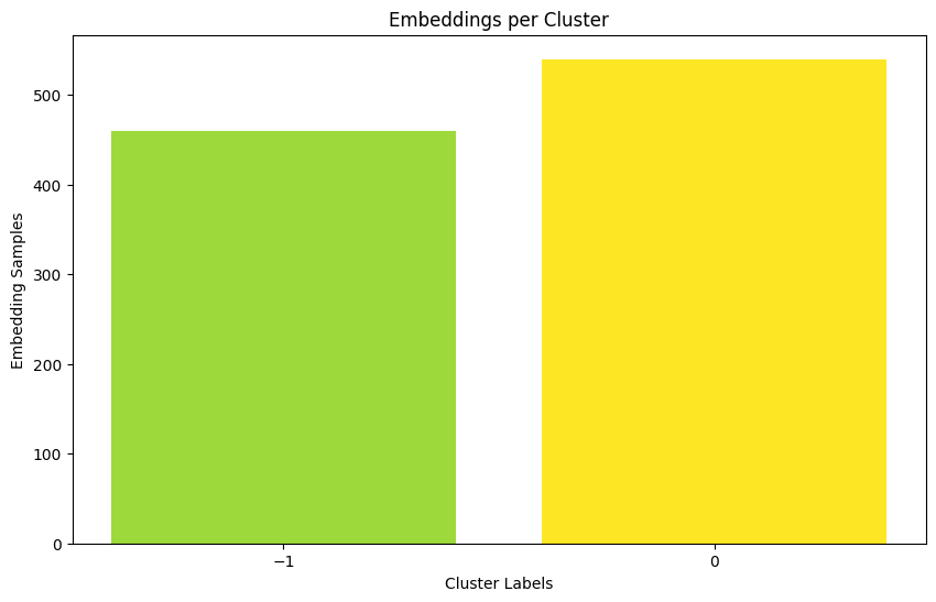
DBSCAN

Script extracted from RAPIDS API tutorial.

More information available at: https://docs.rapids.ai/api/cuml/stable/api/#clustering

%%time
ary = cp.asarray(prot_embeddings)
prev_output_type = cuml.global_settings.output_type
cuml.set_global_output_type('cudf')
dbscan_float = cuml.DBSCAN(eps=0.05, min_samples=100)
dbscan_float.fit(ary)
cuml.set_global_output_type(prev_output_type)
print("Num. Of Clusters: ", dbscan_float.labels_.nunique())

import matplotlib.ticker as ticker
labels = dbscan_float.labels_.values.get()

# Count the number of samples in each cluster
unique_labels, counts = np.unique(labels, return_counts=True)

# Plot the histogram
plt.figure(figsize=(10, 6))
plt.bar(unique_labels, counts, color=plt.cm.viridis(counts / float(max(counts))))
plt.xlabel('Cluster Labels')
plt.ylabel('Embedding Samples')
plt.title('Embeddings per Cluster')

# Ensure all labels are displayed on x-axis and they are integers
ax = plt.gca()
ax.xaxis.set_major_locator(ticker.MaxNLocator(integer=True))
ax.set_xticks(unique_labels)

plt.show()

Num. Of Clusters:  2

../_images/948daa4563a91a07800db57e513ac0c99d37ff42b0adf0589257572444565bd4.png

CPU times: user 109 ms, sys: 143 ms, total: 253 ms
Wall time: 110 ms

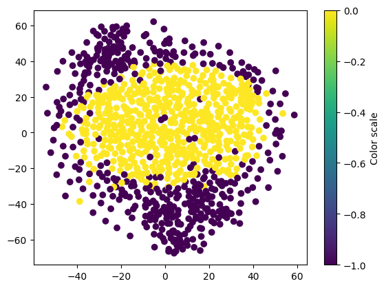
Using T-SNE to reduce dimensionality so that we can visualize the clusters of data

%%time
# Hyperparameters picked arbitrarily for this example
tsne = cumlTSNE(n_components=2, perplexity=20, learning_rate=300, random_state=42)
tsne_embedding = tsne.fit_transform(ary)

# Create scatterplot
colors = dbscan_float.labels_.values.get()
plt.scatter(tsne_embedding.iloc[:,0].to_numpy(), tsne_embedding.iloc[:,1].to_numpy(), c=colors)
# Add a colorbar
plt.colorbar(label='Color scale')
# Show plot
plt.show()

../_images/c5304a408332087a2d1338418a1ac2ba51810e402de8e4573303ed6be84e90df.png

CPU times: user 1.91 s, sys: 471 ms, total: 2.38 s
Wall time: 3.3 s

The plot above is for the sake of exemplification based on a subset of random proteins and should not be representative of a full application.

Conclusion#

In this example, you saw how simple it is to operate with BioNeMo and integrate it with classic clustering and dataframe manipulation activities.

NVIDIA BioNeMo Framework

Generating Embeddings for Protein Clustering

Contents

Generating Embeddings for Protein Clustering#

Prerequisites:#

Download the Pre-trained Models#

Run the container#

Download the data#

Using BioNeMo features to download UniRef50#

Alternative datasets#

Generating Embeddings#

Example#

ESM-1nv limits#

Data Cleaning#

Conclusion#