MeshGraphNet: A Practical User Tutorial#

Welcome to this in-depth technical tutorial on the MeshGraphNet (MGN) model. This guide is designed to help you understand the core architecture of this powerful Graph Neural Network, its specialized variants, and the suite of high-performance optimizations available in the PhysicsNeMo library. By the end of this tutorial, you’ll have a solid grasp of how to use, customize, and optimize the MeshGraphNet for your physical simulation tasks.

The Foundational Architecture#

At its core, MeshGraphNet is a deep learning model that learns to simulate physical systems by processing data represented as a graph. It operates in three sequential and distinct stages:

Encoder
Processor
Decoder

This modular design provides a clean, interpretable pipeline for learning complex, non-linear dynamics directly from data, bypassing the need for explicit governing equations like those used in the Finite Element Method (FEM) or Finite Difference Method (FDM).

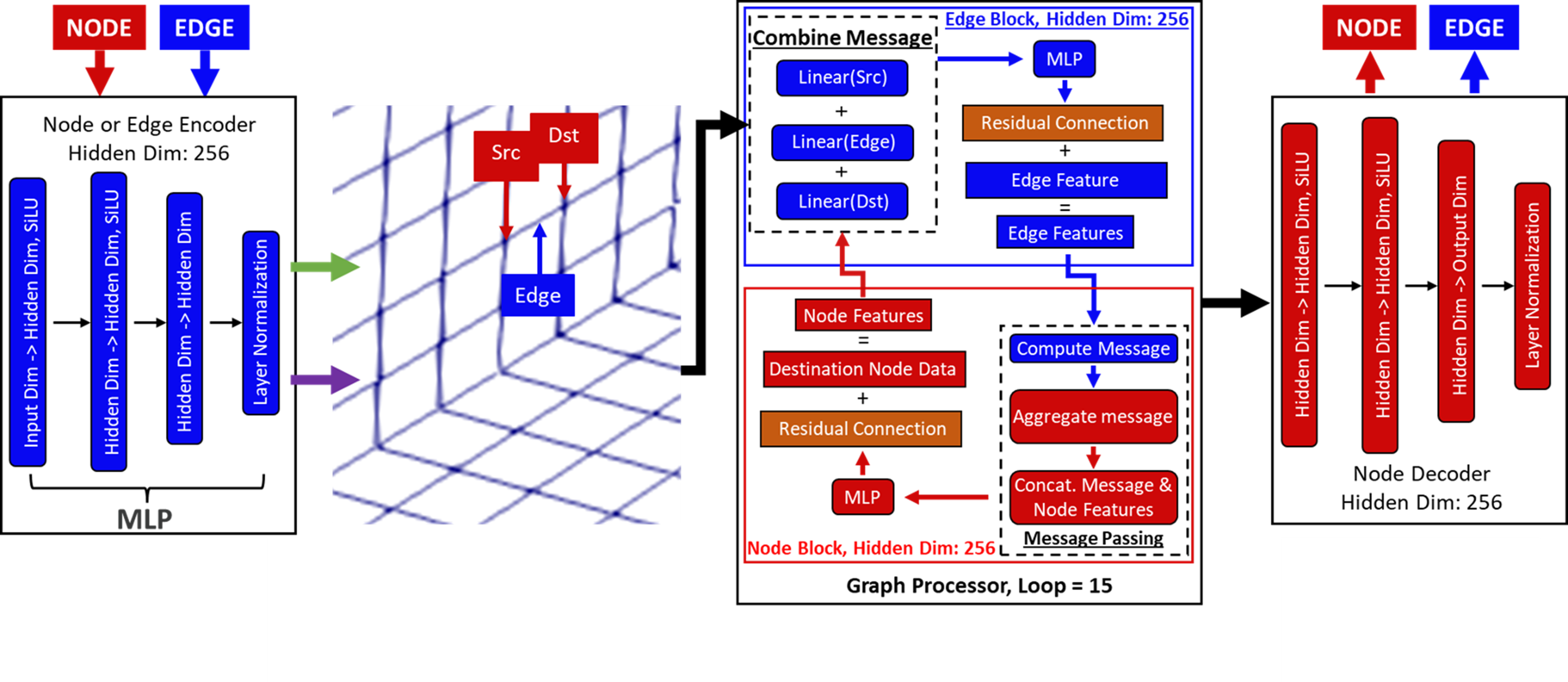
![The MeshGraphNet Architecture](./mgn_architecture.png)

Graph Construction from Simulation Mesh to GNN Input#

The first step in any MeshGraphNet workflow is to convert the physical simulation data, typically represented as a mesh, into a graph structure that the neural network can process. This graph is a rich representation of the system, encoding not just its shape, but also its dynamic physical state at a given moment in time.

The conversion process involves defining the graph’s fundamental components—its nodes and edges—and assigning meaningful feature vectors to each.

The translation from mesh vertices to graph nodes is direct and intuitive.

Rule: Every vertex (point) or cell center in the simulation mesh becomes a single node in the graph.
Node Features: Each node is assigned a feature vector that describes its physical state, such as position, velocity, one-hot encoding of the node type. This vector is assembled from various physical quantities associated with that point in the simulation.

This process results in a set of nodes, each with a feature vector representing the state of a specific point in the physical system.

Edges define the relationships and potential interactions between the nodes:

Rule: Mesh edges are created directly from the mesh’s topology. An edge is drawn between two nodes if their corresponding vertices are connected in a mesh element (for example, the side of a triangle or tetrahedron).
Edge Features: The feature vector for a mesh edge typically contains relational information, such as the displacement vector and Euclidean distance between the two connected nodes.

The result of this construction process is a graph object, populated with nodes and two sets of edges, where each component has a feature vector describing its physical state. This graph is the final input, ready to be passed to the encoder module.

Encoder from Embedded Features to Latent Embeddings#

The Encoder acts as the initial interface, converting raw, heterogeneous physical attributes into a unified, high-dimensional representation. Its primary function is to create rich embedding vectors for both the nodes and the edges of the graph. This is a crucial step because it transforms disparate physical quantities (like position, velocity, and material type) into a unified, abstract feature space where the GNN can more effectively learn patterns and relationships. The MLPs in this stage function as learned feature extractors, automatically discovering the most salient properties from the raw input data.

Node Encoder: A Multi-Layer Perceptron (MLP), typically with ReLU activations, takes the initial node features and maps them to a dense, abstract embedding vector. For example, for transient fluid simulation, the node encoder learns to project its state—position, velocity, pressure, and density—into a latent space that is more informative for the subsequent message-passing process. Importantly, the non-linear transformations of the MLP allow it to capture complex relationships between features.
Edge Encoder: A separate MLP processes relational edge features. These features describe the connection between two nodes. Common features include the displacement vector, and the scalar distance between nodes. This process produces a dedicated edge embedding.

The output of the Encoder is a transformed graph where every node and edge has an enriched embedding vector, ready for the iterative process of information propagation.

Processor as the Message-Passing Engine#

The Processor is the computational heart of the model. It consists of a stack of GNN layers, typically 10-15 layers deep, which iteratively simulate physical interactions by passing and aggregating information across the graph. Each layer contains two interconnected blocks that follow a “gather-combine-update” paradigm:

Edge Block: This block processes every edge in the graph. For each edge, an MLP takes the current edge embedding and the embeddings of its connected source and receiver nodes. It combines this information by concatenation to produce a new, updated edge embedding. This can be seen as the “gather” and “combine” stage, where a message is created based on the states of the interacting particles. The MLP here learns a function that determines the new state of the interaction based on the current states of the two nodes it connects.
Node Block: After the edge embeddings are updated, this block aggregates the messages from all incoming edges. This is typically done by summing or averaging the updated edge embeddings. For a graph node, this aggregation step effectively sums up all the influences from its neighbors. This is the “update” stage. A final MLP then updates the node’s embedding based on its previous state and the newly aggregated message.

By stacking multiple Processor layers, the model’s receptive field expands. Each successive block allows information to travel one more hop across the graph, enabling the model to simulate effects like pressure waves or gravitational forces that extend over large distances. A deep network with 15 processor blocks allows a node to be influenced by other nodes up to 15 hops away, a powerful capability for modeling complex system dynamics. The number of layers directly controls the reach of information. A network that is too shallow might fail to capture long-range effects, while one that is too deep can be computationally expensive and may suffer from over-smoothing, where node features become too similar and lose local distinction.

Decoder from Latent State to Physical Output#

The Decoder is the final component, translating the rich, high-level embeddings from the Processor back into a meaningful physical prediction. A final MLP takes the updated node embeddings and outputs the predicted change in a physical quantity for each node. This is most commonly the change in the physical field, such as the change in velocity and pressure from the current time step to the next time step in transient fluid simulation. This approach of predicting a change (or residual) is more numerically stable than predicting the absolute next state. It helps the model focus on the subtle dynamics rather than the overall system state, making it less prone to accumulating errors over a long simulation. For example, the new velocity of a node at time (t+1) is calculated as its current velocity at time t plus the predicted velocity delta from the decoder.

Architecture Variants#

The PhysicsNeMo library offers several specialized MeshGraphNet variants, each tailored for different simulation needs.

[Base MeshGraphNet](https://github.com/NVIDIA/physicsnemo/blob/main/physicsnemo/models/meshgraphnet/meshgraphnet.py):
The standard model with a single, unified message-passing pipeline. It is the most common choice for general-purpose modeling with GNNs. It is highly customizable, allowing you to set the number of processor blocks (processor_size), hidden dimensions, and activations.
[HybridMeshGraphNet](https://github.com/NVIDIA/physicsnemo/blob/main/physicsnemo/models/meshgraphnet/hybrid_meshgraphnet.py):
This variant is designed for systems with transient physics, accompanied by large deformation. For example, a car crashing into a stiff wall. At each time step, the graph will consist of two edge types:
Mesh edges, representing the node connectivity based on the mesh topology.

World edges, representing the node connectivity based on the current node positions.
This model uses separate encoders for these different edge types and a corresponding hybrid processor to handle them distinctly. Its forward signature requires separate mesh_edge_features and world_edge_features, allowing it to learn distinct dynamics for each type of interaction.

[MeshGraphKAN](https://github.com/NVIDIA/physicsnemo/blob/main/physicsnemo/models/meshgraphnet/meshgraphkan.py):: An experimental variant that replaces the standard node encoder MLP with a Fourier Kolmogorov–Arnold Network (Fourier KAN). KANs are a new type of neural network that theoretically offer richer, more expressive non-linear representations than traditional MLPs. For some problems, this can improve the model’s ability to learn complex dynamics and capture non-monotonic relationships, potentially leading to faster convergence or higher accuracy on specific tasks.
[BiStrideMeshGraphNet](https://github.com/NVIDIA/physicsnemo/blob/main/physicsnemo/models/meshgraphnet/bsms_mgn.py):: This is a multi-scale variant that extends the base model with a U-Net style refinement module. It creates a graph pyramid, which consists of multiple levels of the graph at different resolutions. The model applies a bi-stride message-passing component over these levels to capture both local, fine-grained features and global, coarse-grained features more effectively. This is particularly useful for simulations where having a large receptive field in message passing is important. The bi-stride approach allows the model to efficiently propagate information across large distances.
[X-MeshGraphNet](https://github.com/NVIDIA/physicsnemo/tree/main/examples/cfd/external_aerodynamics/xaeronet/surface):: The Base MeshGraphNet model, and more generally GNNs, face some limitations, including scalability issues, requirements for meshing at the inference, and challenges in handling long-range interactions. X-MeshGraphNet is scalable, multi-scale extension of MeshGraphNet designed to address these challenges. X-MeshGraphNet overcomes the scalability bottleneck by partitioning large graphs and incorporating halo regions that enable seamless message passing across partitions. This, combined with gradient aggregation, ensures that training across partitions is equivalent to processing the entire graph at once. To remove the dependency on simulation meshes, X-MeshGraphNet constructs custom graphs directly from tessellated geometry files (for example, STLs) by generating point clouds on the surface or volume of the object and connecting k-nearest neighbors. Additionally, the model builds multi-scale graphs by iteratively combining coarse and fine-resolution point clouds, where each level refines the previous, allowing for efficient long-range interactions. X-MeshGraphNet maintains the predictive accuracy of the full-graph MeshGraphNet, while significantly improving scalability and flexibility. The use of halo regions and gradient aggregation ensures that the partitioning does not compromise the accuracy, making it equivalent to training on the full graph while significantly reducing memory and computational overhead. See the [X-MeshGraphNet paper](https://arxiv.org/pdf/2411.17164) for more details.

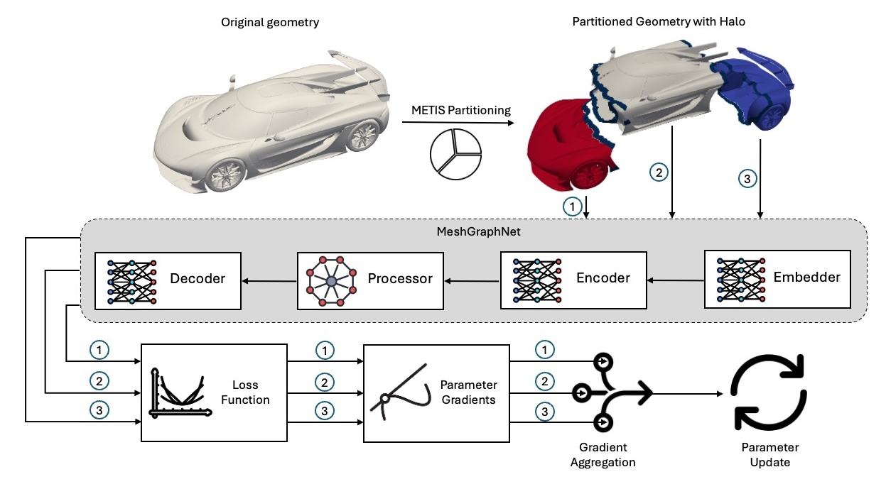
![The X-MeshGraphNet Architecture](./xmeshgraphnet_architecture.jpg)

Optimization Suite#

The PhysicsNeMo library includes several built-in optimizations for MeshGraphNet and its variants to improve training and inference performance, especially on modern NVIDIA GPUs:

Gradient Checkpointing (``num_processor_checkpoint_segments``):
For very deep networks or large graphs, GPU memory can become a bottleneck. Gradient checkpointing is a technique that saves memory by trading a small amount of compute time. Instead of storing all intermediate activations from the forward pass, it recomputes them on the fly during the backward pass. This is especially useful for deep processors where the memory required to store activations would exceed the GPU’s capacity. You can also offload these tensors to the host memory using checkpoint_offloading instead of recomputing activations. This is especially useful for improving performance on Blackwell architectures with fast host-device transfers.

![Memory and performance trade-offs between activation checkpointing and activation checkpointing with offloading](./checkpoint_offloading_performance_comparison.png)
Concatenation Trick (``do_concat_trick``):
A performance optimization that addresses a common bottleneck in GNNs. Concatenating node features to edge features can be slow and memory-intensive. This trick replaces the inefficient concat + MLP pattern with a more efficient MLP + index + sum operation. By avoiding a large memory allocation and copy, it can significantly speed up the processor blocks.
Activation Recomputation (``recompute_activation``):
A more granular memory-saving technique that recomputes activations within individual MLPs. This targets just the non-linear activation function’s output, unlike checkpointing, which recomputes entire layers. It’s a fine-tuned optimization that can provide memory benefits at the cost of some additional computation. This is supported only for SiLU activation.
Optimized Layernorm (``norm_type``): The norm_type parameter allows you
to select between standard “LayerNorm” or the NVIDIA-optimized “TELayerNorm”, which leverages Tensor Cores for faster computation. Tensor Cores are specialized hardware units on NVIDIA GPUs that perform matrix multiplication operations at a high speed. The model automatically falls back to “LayerNorm” on CPUs, ensuring portability.

API and Quickstart#

The following code snippets demonstrate how to get started with the MeshGraphNet family of models.

# Install the necessary libraries. # Ensure Torch is installed with CUDA support, if you have a GPU. # DGL is being deprecated, use PyG (torch-geometric) for new projects. # Do the pip install:

pip install torch torch-scatter torch-geometric physicsnemo

import torch
from torch_geometric.data import Data
from physicsnemo.models.meshgraphnet import MeshGraphNet, HybridMeshGraphNet, MeshGraphKAN, BiStrideMeshGraphNet

# --- Minimal PyG Example (Base MeshGraphNet) ---

# Create a toy graph and random features
# In a real application, these would come from your mesh data
num_nodes = 100
num_edges = 300
edge_index = torch.randint(0, num_nodes, (2, num_edges))
node_features = torch.randn(num_nodes, 4)  # [N, input_dim_nodes]
edge_features = torch.randn(num_edges, 3)  # [E, input_dim_edges]

# Instantiate the base model
model = MeshGraphNet(
    input_dim_nodes=4,
    input_dim_edges=3,
    output_dim=2,
    processor_size=10,
    mlp_activation_fn="relu",
    aggregation="sum",
)

# Run a forward pass
node_outputs = model(node_features, edge_features, edge_index)  # [N, 2]
print("Base MeshGraphNet Output Shape:", node_outputs.shape)
# Output: Base MeshGraphNet Output Shape: torch.Size([100, 2])

# --- HybridMeshGraphNet Example ---
# The Hybrid model requires separate features for mesh and world edges
mesh_edge_features = torch.randn(edge_index.size(1), 3)
world_edge_features = torch.randn(edge_index.size(1), 3)

model_hybrid = HybridMeshGraphNet(input_dim_nodes=4, input_dim_edges=3, output_dim=2)
node_outputs_hybrid = model_hybrid(node_features, mesh_edge_features, world_edge_features, edge_index)
print("HybridMeshGraphNet Output Shape:", node_outputs_hybrid.shape)
# Output: HybridMeshGraphNet Output Shape: torch.Size([100, 2])

# --- MeshGraphKAN Example ---
model_kan = MeshGraphKAN(
    input_dim_nodes=4,
    input_dim_edges=3,
    output_dim=2,
    processor_size=10,
    num_harmonics=5,  # KAN-specific parameter
)
node_outputs_kan = model_kan(node_features, edge_features, edge_index)
print("MeshGraphKAN Output Shape:", node_outputs_kan.shape)
# Output: MeshGraphKAN Output Shape: torch.Size([100, 2])

# --- BiStrideMeshGraphNet Example ---
# This model requires a pre-computed graph pyramid
# In a real-world scenario, you would create these based on your mesh hierarchy
ms_edges = [torch.randint(0, 100, (2, 50)), torch.randint(0, 100, (2, 25))]
ms_ids = [torch.arange(100), torch.arange(50)] # Illustrative
model_bistride = BiStrideMeshGraphNet(
    input_dim_nodes=4, input_dim_edges=3, output_dim=2, processor_size=10
)
node_outputs_bistride = model_bistride(
    node_features, edge_features, edge_index, ms_edges=ms_edges, ms_ids=ms_ids
)
print("BiStrideMeshGraphNet Output Shape:", node_outputs_bistride.shape)
# Output: BiStrideMeshGraphNet Output Shape: torch.Size([100, 2])

Enabling Optimizations Examples#

# Enable common performance optimizations in MeshGraphNet
model_opt = MeshGraphNet(
    input_dim_nodes=4,
    input_dim_edges=3,
    output_dim=2,
    processor_size=10,
    mlp_activation_fn="silu",
    aggregation="sum",
    # Optimizations
    num_processor_checkpoint_segments=2,
    checkpoint_offloading=True,
    do_concat_trick=True,
    recompute_activation=True,
    norm_type="TELayerNorm",
)

node_outputs_opt = model_opt(node_features, edge_features, edge_index)
print("Optimized MeshGraphNet Output Shape:", node_outputs_opt.shape)

Modifying and Customizing the Architecture#

The modular design makes it easy to customize the model’s components. You can create your own modules and swap them into the main architecture by subclassing the base model. This is especially useful for implementing custom message-passing logic or replacing components with novel designs.

Implementing a Custom Processor with Residual Connections#

import torch.nn as nn
from physicsnemo.models.meshgraphnet import MeshGraphNet
from physicsnemo.models.gnn_layers import MeshEdgeBlock, MeshNodeBlock

# Create a custom processor that uses a residual connection
class ResidualProcessor(nn.Module):
    def __init__(self, num_blocks, node_dim, edge_dim, **kwargs):
        super().__init__()
        # Create a list of blocks with residual connections
        self.blocks = nn.ModuleList([
            nn.ModuleDict({
                "edge": MeshEdgeBlock(
                    input_dim_node=node_dim,
                    input_dim_edge=edge_dim,
                    **kwargs
                ),
                "node": MeshNodeBlock(
                    input_dim_node=node_dim,
                    input_dim_edge=edge_dim,
                    **kwargs
                ),
            }) for _ in range(num_blocks)
        ])

    def forward(self, node_x, edge_e, graph):
        for b in self.blocks:
            # First, update the edge features
            edge_e = b["edge"](node_x, edge_e, graph)
            # Then, update the node features with a residual connection
            node_x = node_x + b["node"](node_x, edge_e, graph)
        return node_x

# Subclass MeshGraphNet and swap in the custom processor
class MyMeshGraphNet(MeshGraphNet):
    def __init__(self, **kwargs):
        # The parent constructor builds the encoders and decoder
        super().__init__(**kwargs)
        # Override the default processor with our custom one
        self.processor = ResidualProcessor(
            num_blocks=kwargs.get("processor_size", 15),
            node_dim=self.node_encoder.output_dim,
            edge_dim=self.edge_encoder.output_dim,
            **kwargs
        )

# Example Usage
# This will now use your custom processor with residual connections
model_custom = MyMeshGraphNet(
    input_dim_nodes=4,
    input_dim_edges=3,
    output_dim=2,
    processor_size=10,
    mlp_activation_fn="gelu",
)

# Run a forward pass with the custom model
node_outputs_custom = model_custom(node_features, edge_features, edge_index)
print("Custom MeshGraphNet Output Shape:", node_outputs_custom.shape)
# Output: Custom MeshGraphNet Output Shape: torch.Size([100, 2])