Uncertainty Quantification#

A typical neural surrogate returns a prediction for any input you give it. It provides no estimate of how confident the model is in that prediction. A model running on inputs far from its training distribution is likely to produce an incorrect result, and the model itself has no way to convey that. Uncertainty quantification (UQ) supplies the missing second output: an estimate of how wrong each prediction is likely to be.

This page explains the methods and utilities available in PhysicsNeMo for quantifying that uncertainty, and how to add them to your existing recipe. A well-calibrated uncertainty indicates where to trust the model, helps detect out-of-distribution (OOD) inputs, and drives downstream workflows such as Active Learning.

Warning

Some functionalities discussed here live in physicsnemo.experimental.uq and are an experimental feature. APIs and functionality may change in future releases without backward compatibility guarantees. Contributions are welcome.

Why Quantify Uncertainty#

In scientific and engineering applications, a surrogate is typically deployed in scenarios where no ground truth exists. Without a reference solution, and without a domain expert to review every result, a deterministic prediction carries no signal about whether you should trust it. The Guardrails in PhysicsNeMo catch part of the problem. They screen an input before inference, and they test a prediction against the governing equations afterward with the residual utilities from Physics-guided. Those checks still leave gaps. A high physics residual marks a prediction as suspect, and a low one does not establish that the prediction is right. Training data that itself carries finite residuals weakens the signal further. An input screen, in turn, misses failures that arise in the downstream layers of the model. A model that reports its own confidence score is valuable in its own right. In most cases, that confidence takes the form of a model variance. A high reported variance at a point means the model could plausibly have produced noticeably different outputs there, which is a signal to place less trust in the prediction.

A deterministic prediction also cannot help in the scenarios below:

Unfamiliar input. A model trained on one family of inputs produces a plausible prediction on an input the training never covered. For example, a model trained on one vehicle body style produces a plausible pressure field on a different body style at a much larger error. The output looks no different from an accurate prediction.
Uneven error distribution. Within a single inference, the prediction can be accurate in some regions and much less accurate in others. A model predicting the flow around an object may capture the upstream flow well. The same prediction can still carry large errors in the regions of interest: the wake and the boundary layers.

Uncertainty estimates address these shortcomings. As with evaluating a deterministic model, no single metric captures every effect, so different failure modes need uncertainty reported at different scopes.

What Uncertainty Means for an Input-Conditioned Surrogate#

A probabilistic surrogate returns a predictive distribution for each point and channel, rather than one value. Under a Gaussian assumption, that distribution reduces to a mean and a standard deviation. The mean plays the role of the deterministic prediction, and the standard deviation carries the new information.

Common Uncertainty Scopes#

Uncertainty questions arise at more than one scope. This page covers the four below, which need different tools and different evaluation:

Scope	Question	Where to look
Input	Is this input one the model can handle at all?	Guardrails covers input screening and OOD detection
Whole prediction	Should you trust this prediction as a whole, before asking which parts?	Uncertainty pooled over the case, as in Out-of-Distribution Behavior
Local prediction	Which regions of this prediction should you distrust?	Per-point standard deviation from the methods on this page
Derived quantity	How wide is the interval on the number you report, for example a drag coefficient?	Prediction uncertainty propagated through the derived quantity

The Variance Decomposition#

Split the predictive variance into two parts that answer different questions:

total_variance(x)  =  epistemic_variance(x)  +  sigma^2(x)
                      ^^^^^^^^^^^^^^^^^^^^^     ^^^^^^^^^^
                      model uncertainty         input-dependent
                                                observation noise

Use the epistemic part for maps of where the model is unsure, for OOD detection, and for active-learning acquisition. By definition, this part covers what more training data near the input in question can reduce. Use the total variance for prediction intervals and for calibration metrics, since that is the width an interval has to cover.

Methods differ in which parts they report. They also differ in whether their epistemic estimate carries any notion of distance from the training data:

The variational Gaussian process heads described later return both terms separately from one forward pass. The kernel compares an input against stored reference points, so the epistemic term carries an explicit measure of distance.
Monte Carlo dropout and ensembles measure the spread across stochastic passes or members. That spread estimates the epistemic part alone, unless you add a separate noise output to the model. It reports how much the sampled networks disagree at that input. Nothing in it refers to the training inputs, so the spread can stay narrow on an input the model never saw. Confirm the OOD behavior of such an estimate on held-out unfamiliar cases.
A plain mean-variance network trained on a Gaussian likelihood returns the total only.

How to read the second term depends on your data:

On deterministic simulation data, it measures model discrepancy. Machine learning literature splits predictive uncertainty into two parts. The aleatoric part covers irreducible randomness in the data-generating process, which more data cannot remove. The epistemic part covers ignorance about the model, which more data does reduce. That split assumes noisy observations of some underlying truth. Typically, steady Reynolds-averaged Navier-Stokes (RANS) data carries no noise term at all. One geometry maps to exactly one field, and running the case again reproduces it. No aleatoric component exists to estimate, so whatever the model fits in that slot measures something else. It absorbs the part of the residual that the model’s mean cannot represent. That makes it a learned model-discrepancy variance. The idea comes from Bayesian calibration of computer models, which added a discrepancy term for this purpose. The term covers the mismatch that remains once the model fits as well as it can. It maps where the surrogate is structurally wrong. That reading is also the more useful one, because a map of structural error points at what to fix in the model.

On genuinely noisy data, the term carries its conventional meaning. Some targets do carry real observational scatter, from experimental measurements, a stochastic solver, or a simulation averaged over a finite window. Aleatoric uncertainty then has physical meaning for your problem, and the same machinery captures it with no code change. The noise head is the standard heteroscedastic-GP estimator for exactly that quantity.

The mechanism stays conventional either way, following Kendall and Gal (2017). A small network predicts the noise scale from the same features the kernel uses, trained through a noise-attenuated Gaussian likelihood. Only the interpretation depends on the dataset.

Methods Available in PhysicsNeMo#

Method	Kind	Granularity	Inference cost	Location
`VariationalGPHead`	Closed-form	One scalar per geometry	One pass	`physicsnemo.experimental.uq`
`FieldVariationalGPHead`	Closed-form	Per point, per channel	One pass	`physicsnemo.experimental.uq`
`ConcreteDropout`	Sampling	Per point, per channel	20 to 30 stochastic passes	`physicsnemo.nn`
Ensembles	Sampling	Per point, per channel	One pass per member	Recipe pattern

PhysicsNeMo provides two Gaussian Process (GP) heads that are siblings on the same variational-GP machinery. The scalar head pools a geometry into one embedding and predicts one quantity, such as a drag coefficient. The field head keeps the point dimension and predicts every channel of the field.

Both GP heads require GPyTorch:

pip install nvidia-physicsnemo[uq-extras]
# or simply:
pip install gpytorch

Closed-Form and Sampling Methods#

The kind column carries the main practical axis, and it sorts almost every mainstream UQ method rather than only the four above. The evaluation framework uses the same two names for the UQ_METHOD value a model wrapper declares.

Kind	What it does	Other methods in the same family
`closed_form`	Emits the distribution parameters directly, so one forward pass returns the prediction and its uncertainty together. In exchange, it changes how you train.	Mean-variance networks, evidential deep learning, distance-aware deterministic networks, quantile regression
`sampling`	Builds the distribution from statistics over repeated evaluations. Training stays almost untouched, and you pay for the extra passes instead.	Weight-space Bayesian methods such as variational inference and Markov chain Monte Carlo, test-time augmentation

Predictive UQ is a large field, and the methods on this page are a small selection from it. Post-hoc calibration methods fall outside the split, because they transform a predictive distribution that already exists, using held-out data. Conformal prediction, temperature scaling, and isotonic recalibration all work that way.

Choosing a Method#

Method	Training cost	Inference cost	Difficulty to get right
GP head	Slightly above deterministic	One pass	High
Concrete dropout	Close to deterministic	20 to 30 passes	Low
Ensembles	One run per member	One pass per member	Low

A GP head returns a distance-aware variance from a single pass, so it costs the least at inference. The scale of that variance follows from the recipe and from the train-to-deployment shift. Check it on held-out cases before reading it as an error bar. Training the head demands the most care of the three methods. The recipe carries genuine requirements, and skipping them yields a collapsed or diverged variance rather than a merely mediocre one. Concrete dropout trains almost like a deterministic model and pays at inference instead, which makes it the sampling option when K trainings are out of reach. Ensembles need no change to the model or the loss, and pay at training time.

Tip

Decide which property you need before you compare methods. A method that looks stronger on one uncertainty metric can look weaker on another, because calibration, error ranking, and OOD behavior are different properties. PhysicsNeMo-CFD carries an evaluation framework and metric suite for running that comparison on your own data. Refer to Evaluating Uncertainty.

Adding UQ Capabilities to an Existing Model#

Every method below provides guidance on: when to use it, what it assumes, training, inference, calibration, cost, and limitations.

The commands come from the external aerodynamics transformer models recipe. That recipe implements every method here on a GeoTransolver backbone.

Concrete Dropout#

Use it when you want a sampling-based estimate without a deep ensemble’s training cost. One run produces the model, and the members become stochastic passes at inference, so the training budget stays at one model rather than K. It suits a backbone that already applies dropout, where the change stays local: swap those layers and add one term to the loss. The cheaper ensemble variants also cost about one run. This method keeps a single checkpoint, though, and lets you choose the sample count at inference rather than fixing it during training.

What it assumes. Dropout left active at inference approximates a variational posterior over the weights, so the spread across passes stands in for model uncertainty. That spread covers the epistemic part alone, and it carries no measure of distance from the training data. Stable per-point moments also assume enough passes.

Ordinary Monte Carlo dropout asks you to choose the per-layer dropout rate by hand. That rate sets the size of the uncertainty you get back, so an arbitrary hyperparameter decides your error bars. Concrete dropout makes the dropout probability learnable through a continuous relaxation of the Bernoulli mask. Each layer then fits its own rate during training, and a regularization term keeps that rate away from the degenerate values of zero and one. Hand-tuning is impractical at this scale, because a sweep over per-layer rates means repeated multi-GPU trainings. Inference costs the same either way, so this is a better-conditioned version of the same method rather than a different one.

Training. On GeoTransolver, enable it with two settings:

python src/train.py --config-name geotransolver_surface \
    model.concrete_dropout=true \
    training.lambda_reg=1e-4

model.concrete_dropout=true replaces the standard dropout layers with learnable ConcreteDropout layers. training.lambda_reg is the coefficient on the dropout entropy regularization. It defaults to 0.0, which turns the term off, and useful values run from 1e-5 to 1e-3. Training logs the learned rates under dropout_rates/.

Inference. Run with a chosen number of stochastic passes:

python src/inference_on_zarr.py --config-name geotransolver_surface \
    run_id=/path/to/model/ \
    mc_dropout_samples=20

Calibration. Nothing in the method sets the scale of the spread against observed error, so treat calibration as something to measure rather than to expect. The spread reports the epistemic part alone, which tends to sit below the total error. Recalibrate on held-out data, or add a noise output for the rest. Too few passes bias the per-point standard deviation downward as well.

Cost. Training costs close to the deterministic model. Inference costs one full pass per sample, so 20 to 30 passes per case.

Limitations. The spread carries no distance awareness, so it can stay narrow on an input the model never saw. Learned rates can collapse toward zero and take the spread with them. The layers are also a no-op in evaluation mode, which fails silently.

Porting it to another model. Models such as GALE and GeoTransolver expose the flag already. Any model that applies dropout can adopt the method through three steps:

Swap the dropout sites. Replace nn.Dropout with ConcreteDropout wherever the model already drops activations. GALE and the GeoTransolver context projector do exactly this at each block’s output projection, and nothing more elaborate. Reuse the existing sites rather than inventing new ones.
Add the regularization loss. collect_concrete_dropout_losses(model) walks the module tree and sums the per-layer terms, so it works wherever the layers ended up. The rates already receive gradients from the prediction loss, so this term is not what makes them learn. It adds the negative entropy of each Bernoulli rate to the loss, which pushes the rate away from zero and one. Without it the learned rates can collapse toward degenerate values, which drains the sample spread and the uncertainty estimate with it.
Restore stochastic sampling at inference. Call model.eval(), then put only the ConcreteDropout modules back into training mode.

import torch
from physicsnemo.nn import (
    ConcreteDropout,
    collect_concrete_dropout_losses,
    get_concrete_dropout_rates,
)

# 1. Swap an existing dropout site.
block.out_dropout = ConcreteDropout(in_features=hidden_dim, init_p=0.05)

# 2. Add the regularization term to the loss.
loss = mse(pred, target) + lambda_reg * collect_concrete_dropout_losses(model)

# 3. Sample at inference: eval mode, then dropout layers back to train mode.
model.eval()
for module in model.modules():
    if isinstance(module, ConcreteDropout):
        module.train()

preds = torch.stack([model(inputs) for _ in range(num_samples)])
mean, std = preds.mean(dim=0), preds.std(dim=0)

Warning

ConcreteDropout is a no-op in evaluation mode, matching nn.Dropout. A Monte Carlo loop that skips step 3 returns a standard deviation of exactly zero at every point, and raises no error. Log the learned rates with get_concrete_dropout_rates(model) as well. Rates that collapse toward zero take the sample spread with them.

The Variational Gaussian Process Head#

Use it when you need per-point uncertainty on a large mesh or point cloud, and one forward pass has to produce it. PhysicsNeMo builds its closed-form UQ utilities on a variational GP because of the properties below, which many surrogate models in science and engineering need:

Distance awareness. The GP posterior variance grows as inputs move away from the inducing points. The uncertainty then follows from how far an input sits from what the model saw. Few alternatives offer that. A mean-variance or evidential network predicts the variance with a network that stays free to be confidently wrong far from the training data. Dropout and ensembles report disagreement among sampled networks, which need not grow on an unfamiliar input either.
One forward pass. Closed-form variance matters on the large meshes and point clouds typical of computational fluid dynamics and computer-aided engineering. At millions of points, 20 to 30 passes per geometry becomes a real operational cost.
An explicit variance split. The GP separates posterior variance from the noise term in closed form. The epistemic part can then drive OOD detection and acquisition while the total drives intervals. Monte Carlo dropout supplies the epistemic part alone, unless you add a separate noise head.

Distance-aware deterministic networks reach the same property by a related route. Deep kernel learning feeding a variational GP is the published construction that FieldVariationalGPHead implements, rather than a new one. Deep kernel learning also carries two documented failure modes: the kernel can fit training features too closely, and the feature space can collapse. Those modes are why the feature normalization and kernel constraints described later are not optional knobs. Quantile regression, conformal prediction, and other post-hoc closed-form methods sit outside the scope of these utilities. Their absence reflects that scope rather than a negative result.

FieldVariationalGPHead replaces a backbone’s final projection with a per-point multitask variational GP. A single forward pass then returns the mean field, the total variance, and the epistemic variance.

What it assumes. Each output channel gets its own variational GP, with a shared inducing-point structure and independent kernels, so the head models no cross-channel covariance. Every point carries a Gaussian likelihood. The kernel’s smoothness parameter sets how many times the sample paths differentiate, which encodes how smooth the head assumes the field to be. The default of 5/2 suits smooth physical fields. It differentiates enough for a pressure or shear field, and stays short of the radial basis function limit, which tends to over-smooth. Automatic relevance determination (ARD) gives every kernel input dimension its own length scale, so growing one length scale switches that feature off. The kernel also assumes its inputs arrive on a fixed scale, which is the job of feature_norm, and that the inducing points cover the feature distribution the backbone produces.

What the head consumes. The head takes a feature tensor and nothing else. It has no dependency on mesh topology, and coordinates are not a separate input, so any positional encoding the backbone applies arrives inside the features. The contract has two parts:

The backbone emits per-point features with last dimension input_dim. The head flattens any leading batch and point dimensions internally, so (B, N, D), (N, D), and (B, T, N, D) all work.
Targets arrive as (..., num_tasks) with matching leading dimensions.

input (mesh, point cloud, graph, ...)
  |
  v
+-------------------+
|   your backbone   |   any point-wise encoder
+-------------------+
  |
  |  features  (B, N, input_dim)
  v
+---------------------------------------------------------+
|                 FieldVariationalGPHead                  |
|                                                         |
|   DKL MLP  ->  feature norm  ->  variational GP         |
|  (mlp_hidden)  (feature_norm)   (n_inducing, num_tasks) |
|                    |                                    |
|                    +---->  noise MLP (noise_mlp_hidden) |
+---------------------------------------------------------+
  |
  v
mean, variance, epistemic_variance   (B, N, num_tasks)

The DKL network compresses the backbone features, and the feature norm puts them in a range the kernel handles well. The noise network branches off the same tensor the kernel receives, so both terms read one shared representation of the input. Both networks are optional. Set mlp_hidden=None to feed backbone features straight to the kernel, and leave noise_mlp_hidden unset for one learned noise scalar per channel instead of a per-point field.

That contract is what makes the head backbone-agnostic. To attach it to DoMINO, MeshGraphNet, or another point-wise encoder, expose whatever the model computes before its final projection.

Training. The example below uses one geometry per step, 12288 sampled points, a 384-wide backbone feature, and four output channels, for example pressure plus three wall-shear components:

import torch
from physicsnemo.experimental.uq import FieldVariationalGPHead

B, N, D, C = 1, 12288, 384, 4        # geometries, points, feature width, channels
M = 1024                             # inducing points per channel

head = FieldVariationalGPHead(
    input_dim=D,                     # backbone feature width
    num_tasks=C,                     # output channels
    n_inducing=M,                    # n_train normalizes the evidence lower bound (ELBO): points per epoch.
    n_train=n_geometries * N,
    mlp_hidden=[128, 16],            # DKL compression, 384 -> 128 -> 16
    feature_norm="l2_radial",        # 16 direction dims + 1 radius dim -> kernel
    noise_mlp_hidden=[64, 64],       # per-point observation noise
    noise_std_range=[0.01, 10.0],    # floor and ceiling on that noise
).to(device)

# Once the backbone is warm, seed the inducing points from real features.
# set_inducing_points expects exactly n_inducing rows, so subsample to M.
with torch.no_grad():
    feats = backbone.encode(batch).reshape(-1, D)     # (B * N, D)
    idx = torch.randperm(feats.shape[0], device=feats.device)[:M]
    head.set_inducing_points(feats[idx])              # (M, D)

# Training step.
feats = backbone.encode(batch)                        # (B, N, D)
targets = batch["fields"]                             # (B, N, C), same leading dims
mean, neg_elbo = head.forward_and_loss(feats, targets, beta=beta)
loss = neg_elbo + lambda_mse * mse(mean, targets)     # mean is (B, N, C)
loss.backward()

The code above runs, but the loss alone does not carry a fresh backbone to a useful field surrogate. The following items belong to the training recipe rather than to the architecture, which is why they live in the training script rather than in the head. They matter more than typical hyperparameters, because the failure they prevent is a collapsed variance or a diverging noise scale rather than a slightly worse model:

Seed the inducing points from real features. The default random inducing points sit nowhere near the backbone’s feature distribution. Push a few batches through the backbone after it warms up, then pass exactly n_inducing of those features to head.set_inducing_points(). The call takes (M, D) or (num_tasks, M, D) in raw feature space. Any other count fails on a shape mismatch. The recipe’s collect_inducing_features helper in src/field_gp_utils.py gathers them across batches.
Anchor the posterior mean with an auxiliary loss. The ELBO can buy likelihood by inflating the variance instead of improving the mean. A mean squared error term on the GP mean removes that shortcut while the backbone still learns the field.
Ramp the KL term. Keep the data-fit term dominant at first, so the mean becomes accurate before the KL term pulls the variational posterior toward the prior. The beta argument to forward_and_loss is that weight.
Add a noise floor and gradient clipping whenever the noise network runs. The ELBO weights each point by 1/sigma^2(x), so a single point whose noise collapses dominates the step. noise_std_range bounds the collapse, and clipping absorbs the correction that follows it.
Set n_train to the number of training points per epoch, meaning geometries multiplied by points per geometry, not the number of geometries. It sets the KL normalization, and a wrong value rescales that term.

The reference recipe configures these terms already. The settled values are the config defaults, so only the data paths and a run identifier need setting:

export PYTORCH_CUDA_ALLOC_CONF=expandable_segments:True
torchrun --nproc-per-node=8 src/train_field_gp.py \
    data.train.data_path=/data/datasets/drivaerstar/surface_files_zarr/class_F/train \
    data.val.data_path=/data/datasets/drivaerstar/surface_files_zarr/class_F/val \
    run_id=geotransolver/surface/field_gp

The keys that change behavior most:

Key	Setting	Purpose
`num_tasks`	`4`	Output channels, such as pressure and three wall-shear components
`n_inducing`	`1024`	Inducing points per task. More points cover feature space better
`mlp_hidden`	`[128, 16]`	Deep kernel learning network that compresses features into the kernel input
`feature_norm`	`l2_radial`	Keeps direction and a standardized radius, so geometry scale stays visible to the kernel
`lengthscale_range`	`[0.01, 2.0]`	Hard bounds per kernel dimension. Prevents a globally smooth kernel with no epistemic contrast
`noise_mlp_hidden`	`[64, 64]`	Network predicting input-dependent observation noise
`noise_std_range`	`[0.01, 10.0]`	Clamp on the noise scale. The floor is load-bearing, not cosmetic
`matern_nu`	`2.5`	Kernel smoothness. The default gives twice-differentiable sample paths
`gp_points_per_step`	`12288`	Points per geometry per step, which bounds the cost of the GP solve

Two of these need retuning on a new dataset. The noise floor works by sitting just below the band the noise head settles into, which depends on how you normalize the targets. Move it with the targets, and check it against the range a run logs. The warmup windows count epochs rather than fractions, so a shorter or longer run needs the window moved.

Inference. One pass returns everything, with no sampling loop:

pred = head.predict(backbone.encode(batch))           # named tuple
pred.mean                # (B, N, C) predicted field
pred.variance            # (B, N, C) total variance, for intervals and calibration
pred.epistemic_variance  # (B, N, C) model term, for OOD and acquisition
pred.lower, pred.upper   # (B, N, C) confidence bounds around the mean

Every returned array carries the shape of the targets, so the mean drops into the place a deterministic prediction occupied and the variance channels travel alongside it. From a trained run:

python src/inference_field_gp.py \
    run_id=geotransolver/surface/field_gp \
    +checkpoint_epoch=100

Calibration. The posterior variance is distance-aware by construction, and not calibrated by construction. Whether its scale matches observed error depends on the recipe and on the train-to-deployment shift. Check it on held-out cases before reading it as an error bar. The correction it needs tends to be modest, because the head fits its variance through a likelihood and so meets observed residuals during training, which a sample spread never does. Use the total variance for interval width and the epistemic term for ranking and OOD work. Refer to Evaluating Uncertainty for the metrics that settle the question.

Cost. Inference costs one forward pass. Training costs somewhat more than the deterministic model, and the GP solve dominates that gap, which is what gp_points_per_step bounds. GP internals run in float64 by default, because short length scales make the inducing-point covariance ill-conditioned in float32, so keep automatic mixed precision off for the GP path.

Limitations. The noise head predicts one number per point, with no uncertainty of its own. The classical treatment puts a second GP over the noise instead. That second GP adds a KL term to the loss, which pulls the noise back toward a prior and stops it from running to extremes. Predicting the noise with a plain network gives up that restraint, which is why noise_std_range and gradient clipping stand in for it. A second GP would cost more than it returns at this scale, because it needs its own inducing points, covariance factor, and KL term. Together those come close to doubling the head’s variational state. Two further limits are worth planning around. The head models no covariance between output channels, so a derived quantity that mixes channels needs care. The recipe items above are load-bearing rather than optional, which makes this the most demanding method here to train.

The GP Head in Action on Three Body Styles#

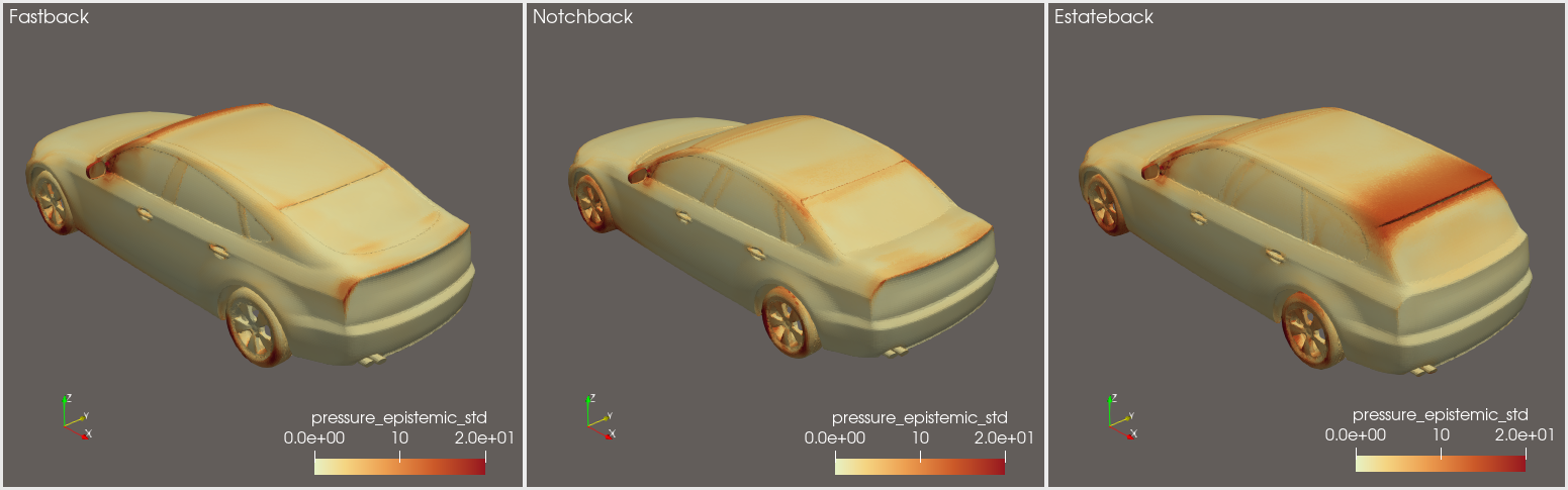
Per-point epistemic standard deviation of surface pressure on three DrivAerStar body styles — Fig. 23 Per-point epistemic standard deviation of surface pressure, from a single forward pass, on three DrivAerStar body styles with a shared color scale.#

The run above used Fastback geometries alone for training, then evaluated the Notchback and Estateback classes. The uncertainty field follows the geometry rather than scattering into per-point noise, and its size tracks geometric similarity to the training set. The Notchback, closest of the three to a Fastback, stays near the in-distribution level. The extended roof and tailgate of the Estateback form the most uncertain region in the figure.

The Scalar Gaussian Process Head#

Use it when the number you report is the deliverable, such as a drag coefficient, a lift coefficient, or a peak stress. VariationalGPHead is the field head’s sibling for that case. It consumes one pooled embedding per sample, of shape (B, input_dim), and returns a mean and a variance per sample.

What it assumes. The same variational-GP assumptions as the field head, with two changes. The geometry has to reduce to one vector, so the pooling layer in front becomes part of the model. The noise is one learned scale rather than a field, since there is one output per case.

The embedding is where the two heads differ in practice. A field head reads per-point features, while this head needs the geometry reduced to one vector, so a pooling layer sits in front of it. physicsnemo.nn.module.pooling provides MeanPooling and AttentionPooling for that step, and the pooling trains jointly with the head.

Training.

from physicsnemo.experimental.uq import VariationalGPHead
from physicsnemo.nn.module.pooling import AttentionPooling

pool = AttentionPooling(feat_dim=384, embed_dim=64)   # (B, N, 384) -> (B, 64)
head = VariationalGPHead(
    input_dim=64,            # pooled embedding width
    n_train=n_geometries,    # one training point per geometry, the ELBO normalizer
    n_inducing=128,
    mlp_hidden=[32, 16],     # optional DKL compression
)

embedding = pool(backbone.encode(batch))                     # (B, 64)
mean, neg_elbo = head.forward_and_loss(embedding, targets)    # targets (B,)

Inference.

pred = head.predict(pool(backbone.encode(batch)))
pred.mean, pred.variance    # (B,) each
pred.lower, pred.upper      # (B,) confidence bounds

Calibration. The same caveat applies as for the field head. Distance awareness does not imply calibration, so check the interval before reading it as an error bar.

Cost. One forward pass, and the pooling layer adds little to it. Training tracks the deterministic model, and the GP solve stays cheap because each case contributes one point rather than a mesh.

Limitations. The head says nothing about the field, so a per-point map needs the field head. Its noise term is one scale for the whole dataset, which cannot express a case that is intrinsically noisier than the rest.

Differences from the field head. Both heads share the same variance structure, a latent GP variance plus an observation-noise term. What differs is how the noise varies across the output. The field head learns a base noise scale per channel, and its noise network modulates that base point by point. The result is a spatially varying version of the same term. Leave noise_mlp_hidden unset and the two heads match, one learned noise scale per output channel. The scalar head predicts one quantity, so it learns one such scale.

The heads differ in what predict packages. The field head returns epistemic_variance next to the total, while GPPrediction from the scalar head carries the total alone. The split stays available either way: forward(embedding).variance is the latent term, and likelihood.noise is the noise the total adds to it.

Three smaller differences remain. n_train counts training geometries here rather than points. Starting inducing points arrive through the inducing_points argument at construction, since this head has no separate seeding call. It also has no feature_norm argument. The pooling layers carry a normalize flag that projects the embedding onto a sphere.

The choice between the two heads is not only about which output you want. A field head plus propagation through a force integral also yields an interval on a coefficient, and Decision-Level Uncertainty explains why that interval is a lower bound. A scalar head learns the variance of the quantity directly instead, and pays for it by predicting nothing about the field. Training both heads on one shared backbone is a practical middle ground. See transformer models recipe for different options. The scalar head also drives the acquisition step in the active learning recipe.

Ensembles#

Use it when you want uncertainty without touching the model or the loss, and you can afford either extra trainings or extra checkpoints. This is the only option here for a model you cannot change.

What it assumes. The spread across members stands in for model uncertainty, so the members have to differ in ways that matter for the prediction. Diversity is the whole mechanism, and it carries no measure of distance from the training data.

Training. An ensemble needs no library support, only more than one set of weights and a rule for combining their predictions. The variants differ in where the diversity comes from and in what they cost:

Variant	How to build it	Diversity source	Cost
Deep ensemble	K independent runs with different seeds for initialization and data order	Different optima	K trainings
Snapshot ensemble	One run with a cyclic learning-rate schedule, saving a checkpoint at the end of each cycle	Basins visited after each learning-rate restart	About one training
Checkpoint ensemble	The last K epochs of a single ordinary run	Late-training weight variation	Free if the run exists
Input ensemble	One model applied to decimated and remeshed variants of one geometry	Input sensitivity rather than weight uncertainty	K inference passes

Diversity decreases down the table, so a checkpoint ensemble costs the least and delivers the least. A snapshot ensemble depends on its cyclic schedule. Without learning-rate restarts it degenerates into a checkpoint ensemble. The input ensemble measures something different again. Refer to Guardrails for that variant.

Inference. One pass per member. When combining members, iterate one member at a time and accumulate running statistics. Memory then stays proportional to one field rather than to K fields.

Calibration. The member spread covers the epistemic part alone, so it tends to fall short of the observed error and needs recalibration on held-out data. A small K also makes the variance estimate noisy, which shows up as unstable calibration numbers rather than as an obvious failure.

Cost. K trainings for a deep ensemble, roughly one for a snapshot ensemble, and nothing beyond the run you already have for a checkpoint ensemble. Inference costs K passes in every variant.

Limitations. No distance awareness, so the spread can stay narrow on an unfamiliar input. The cheaper variants buy their savings with correlated members, which narrows the spread without the model improving. K also bounds what the estimate can resolve, since a handful of members cannot describe a tail.

Evaluating Uncertainty#

Uncertainty quality is not one property. The metrics below answer different questions, so compare methods on the axis that matches your purpose.

Calibration#

Are the predicted uncertainties the right size? A predicted standard deviation claims a specific spread of errors, and “right size” means the errors actually observed match that claim. If a model predicts a standard deviation of 2 Pa at a set of points, then the errors at those points should scatter with a standard deviation near 2 Pa. Predicting 0.2 Pa instead makes the model overconfident, so its intervals miss far more often than they promise. Predicting 20 Pa makes the intervals correct but so wide that they rule nothing out.

Every metric here builds on the standardized residual. For point \(k\) with predicted mean \(\mu_k\), predicted standard deviation \(\sigma_k\), and true value \(y_k\):

\[z_k = \frac{y_k - \mu_k}{\sigma_k}\]

Perfect calibration makes the \(z_k\) behave like draws from a standard normal distribution, so their spread is one.

Calibration z-RMS is the root mean square of the standardized residual. The target is 1.0. Above it the model is overconfident, and below it too timid.

\[\text{z-RMS} = \sqrt{\frac{1}{N}\sum_{k=1}^{N} z_k^2}\]
Coverage at 95 percent is the fraction of points whose error falls inside 1.96 predicted standard deviations. The target is 0.95.

\[\text{coverage}_{95} = \frac{1}{N}\sum_{k=1}^{N} \mathbb{1}\left[\,|z_k| \le 1.96\,\right]\]
Negative log predictive density scores the mean and the standard deviation together under a Gaussian likelihood, so a model cannot improve it by widening intervals alone. Lower is better.

\[\text{NLPD} = \frac{1}{N}\sum_{k=1}^{N} \left[\frac{1}{2}\log\left(2\pi\sigma_k^2\right) + \frac{z_k^2}{2}\right]\]
Sharpness is the mean predicted standard deviation. Among models that are equally well calibrated, the sharper one is more useful, because a narrower interval rules out more. Sharpness also reports in the units of the field, unlike the dimensionless metrics above, so it shows whether an interval is narrow enough to act on. Read it next to a calibration metric, because a model can widen every interval to reach the coverage target.

\[\text{sharpness} = \frac{1}{N}\sum_{k=1}^{N} \sigma_k\]

Multiplying every \(\sigma_k\) by one constant moves every metric above. They measure the size of the error bars, not whether the large ones land where the large errors are.

Error Discrimination#

Does high uncertainty land on high error?

Uncertainty-error rank correlation correlates absolute error with predicted standard deviation, ranking the points within one geometry and then averaging across geometries. Higher is better, and 1.0 means the uncertainty orders the points exactly as the error does.
Area under the sparsification error curve (AUSE) measures the same agreement through the decision it supports, namely discarding the predictions you trust least. Sort the items by predicted uncertainty, remove the most uncertain fraction \(f\), and record the error over what remains. Sweeping \(f\) from 0 to 1 traces the sparsification curve. Sorting by true absolute error instead and repeating the sweep traces the oracle curve, which is the ceiling for any ordering. AUSE is the normalized area between the two curves, so lower is better and zero means the predicted uncertainty ordered the items as well as the error itself.

Both metrics depend only on ordering. Multiplying every uncertainty by a constant leaves them unchanged, so they stay informative even when calibration is poor.

Out-of-Distribution Behavior#

Does uncertainty grow as fast as error does? Compute the growth ratio (sigma_ood / sigma_id) / (rmse_ood / rmse_id), where 1.0 means the uncertainty kept pace with the error. A value below one means intervals that hold in distribution become overconfident outside it. For a complementary view, separate in- from out-of-distribution cases by their mean predicted uncertainty, then score that separation with the area under the receiver operating characteristic curve.

This family matters because post-hoc recalibration cannot fix it. Rescaling uncertainties fitted on in-distribution data leaves the growth ratio untouched.

Decision-Level Uncertainty#

Does field uncertainty produce a useful interval on the quantity you act on? For example, propagate per-point standard deviations through the force integral to get a standard deviation on a coefficient such as drag. Then rank that against the actual coefficient error with the same correlation and AUSE measures.

Warning

Propagating per-point variances independently holds exactly only for spatially uncorrelated uncertainty. Epistemic uncertainty is spatially correlated and dominates a coherent surface integral, so this treatment gives a lower bound on the interval. Read it alongside the field-level epistemic metrics. No UQ method can rank a constant bias in a coefficient either, because no uncertainty estimate orders errors that do not vary. When the coefficient is the deliverable, The Scalar Gaussian Process Head learns its variance directly instead of inheriting it from the field.

The Evaluation Framework#

Comparing UQ methods is harder than comparing deterministic models. One method returns its uncertainty in a single pass and another needs dozens of passes. A comparison written separately for each method tends to encode each method’s own conventions, which stops it from being a fair test. The UQ support in PhysicsNeMo-CFD removes that problem for CFD checkpoints. It extends the deterministic model scoring already in that repository to probabilistic predictions. The same cases, the same normalization, and the same accuracy metrics carry over, with the UQ metrics added alongside them.

The metrics live behind a method-agnostic interface. A model wrapper returns a predictive distribution, and every metric reads that object. The framework then scores a closed-form GP posterior and a 32-pass dropout ensemble on identical terms.

The contract is FieldDistribution. It carries the mean, the total standard deviation, and the epistemic and observation-noise parts when a method has them, all in physical units. Optional samples and quantiles fields serve methods whose predictive law is not Gaussian. Sampling wrappers report no separate noise term, so their total and epistemic values coincide.

A wrapper declares UQ_METHOD as either closed_form or sampling. The framework then either calls the model once, or runs run.uq.num_samples passes and accumulates streaming statistics. A deterministic model declares no UQ support, and its UQ metrics report NaN. That keeps the deterministic contrast visible in the results table.

Enable UQ and list the metrics in the benchmark config:

run:
  uq:
    enabled: true
    num_samples: 32          # stochastic passes for sampling wrappers
    retain_samples: false    # keep raw samples; memory-heavy

metrics:
  - nlpd
  - nlpd_epistemic
  - calibration_zrms
  - coverage_95
  - sharpness_std
  - sharpness_epistemic_std
  - uncertainty_error_spearman
  - uncertainty_error_spearman_epistemic
  - sparsification_ause
  - sparsification_ause_epistemic
  - { name: drag_uq, drag_direction: [1, 0, 0] }

reports:
  visuals:
    - sparsification_plot

Then run the benchmark:

python main.py --config-name=config_uq_surface
# or across GPUs
torchrun --standalone --nnodes=1 --nproc_per_node=8 main.py --config-name=config_uq_surface

To score a UQ method of your own, write one wrapper. Declare the method kind, return a FieldDistribution from decode_distribution, and every metric and the sparsification report apply without further work. The reference wrappers in the repository cover a deterministic baseline, a closed-form GP, a Monte Carlo dropout model, and an ensemble, and serve as templates. Refer to PhysicsNeMo-CFD for more details.

Pitfalls and Practical Guidance#

Monte Carlo dropout returns zero uncertainty in evaluation mode, and raises no error. Refer to the warning under Concrete Dropout.
Calibration and error ranking can peak at different checkpoints. Both can degrade with continued training even while the training loss improves. Select checkpoints on the metric that matches your downstream use.
Normalizing away the feature scale also removes the OOD cue. A kernel needs its inputs on a fixed scale. The direct route is to divide each feature vector by its own length, which also discards that length. Length is often the strongest cue that an input is unusual, because unfamiliar inputs tend to produce features of unusual size rather than merely a different direction. Discard it and every input looks equally familiar to the kernel, so the uncertainty stops varying between inputs. feature_norm="l2_radial" keeps the direction and appends the standardized length as one extra kernel dimension. Prefer it over a plain unit-sphere projection of your own.
A bottleneck before the kernel can compress away what marks an input as unfamiliar. Deep kernel learning is worth its place: it gives the kernel a compact input and keeps the solve affordable. The compression still discards information, and what it drops is not always what you expect. Features that separated familiar from unfamiliar inputs upstream of the bottleneck need not separate them at the kernel input. When a workflow depends on the epistemic term, measure that separability before and after the bottleneck rather than assuming either outcome.
An end-to-end score hides which term earned it. The total predictive uncertainty often flags unfamiliar inputs well, and that result does not establish that the epistemic term did the work. The noise term responds to the same inputs and can carry most of the signal. Score the parts separately before you build a workflow on either one.
Model uncertainty complements the checks in Guardrails rather than replacing them. An input screen runs before inference and needs no prediction. A residual check tests a prediction against the governing equations. A predicted variance reports what the model knows about its own reach. The three fail in different ways and their choice depends on the downstream workflow.

Where to Go Next#

Guardrails for input screening, geometry OOD detection, and physics residual checks.
Active Learning for using uncertainty to select the next geometries to label, and for the query strategies that pair it with random sampling to keep the training set representative.
Model Evaluation and Inference for deterministic accuracy evaluation and inference workflows.
The transformer models recipe for the full training and inference reference. It covers the auxiliary loss terms, learning-rate guidance, and a full reference list for the methods on this page.
PhysicsNeMo-CFD for the benchmarking workflow and the metric implementations.