RANPerf Testbench#

Executive Summary#

RANPerf testbench is a comprehensive framework that provides the methodology, documentation, and tools to Aerial developers for benchmarking their GPU-based RAN implementations.
In a first step, we focus on defining the framework for L1 (PHY layer) implementations, with a key benchmarking performance metric being the cell capacity which is defined as the maximum cell count where all enabled channels are 100% on-time, i.e., when they all meet the latency requirements. We plan to provide gradual upgrades to RANPerf testbench by adding benchmarking tests for different cellular deployment scenarios and framework enhancements.
RANPerf testbench supports seven channels and reference signals - PRACH, PDCCH, PUCCH, CSI-RS, PDSCH, PUSCH, SRS, and SSB - and benchmarks the cell capacity, latency, GPU power, GPU memory, and GPU temperature of the Aerial L1 GPU stack (cuPHY) under peak 5G NR traffic loading.
The benchmarking process is driven by a C++ testbench with a user-friendly Python interface that auto-generates YAML configurations and command lines, with the Python interface being the recommended entry point for benchmarking.
RANPerf testbench defines slot-level processing patterns that are repeatedly executed to measure per-channel latency, on-time (that meets the system’s latency requirements), and steady-state power/memory/temperature.
GPU SM (Streaming Multiprocessor) resources are soft partitioned across channels via NVIDIA MPS or CUDA Green Contexts with detailed per-channel controls.

Introduction#

RANPerf testbench is a comprehensive framework that provides the methodology, documentation, and tools to Aerial developers for benchmarking their GPU-based RAN implementations.

RANPerf testbench enables multiple PHY channels to share the same GPU through NVIDIA Multi-Process Service (MPS) or CUDA Green Contexts. It enables execution of different channel workloads, measurement of the latency of each workload over a specific number of time slots, and visualization of the results. The latency generated from RANPerf testbench refers to the GPU execution time of each channel workload as measured by CUDA events. The setup stage and CPU execution portions are not included in the measured latency. RANPerf testbench also supports Nsight Systems trace collection for profiling.

Before proceeding to the details of the benchmarking details, we note the following:

Throughout the RANPerf testbench document, any text directly related to Aerial SDK folders/subfolders and configuration or command line parameters, e.g., --iterations, is formatted as inline code, where the exact usage of the highlighted text will be clear from the surrounding text, and text related to the Appendices of the document, e.g., Appendix B, is referenced directly.
Please refer to the glossary in Appendix A for definitions of key terms used in the document.
For details on how the supported DL and UL L1 channels can be configured, please see Appendix D (DL and UL channel configuration) for a typical example. For the channel configuration detailed in Appendix D, the associated DL and UL spectral efficiency values are calculated in Appendix E.
When we refer to cuMAC (CUDA-Accelerated MAC) or MAC in the RANPerf testbench documentation, it will be clear from the context which subset of the cuMAC functionality is enabled in the RANPerf benchmarking tests.

Benchmarking Procedure#

The RANPerf benchmarking procedure is visualized in Figure 1 which includes the configuration of system parameters, the generation of test vectors (TVs), see Section 4.2 for their definition details, and the generation of benchmarking KPIs at the output of GPU execution. RANPerf benchmarking generates TVs for benchmarking of GPU-based RAN implementations of the L1 and/or L2 layers, while benchmarking of L1/L2 subsystems or other layers/subsystems is not excluded. For L1 implementations that generate peak traffic loading, Appendix D provides the details of the used system configuration parameters, which represent the most challenging system operation conditions.

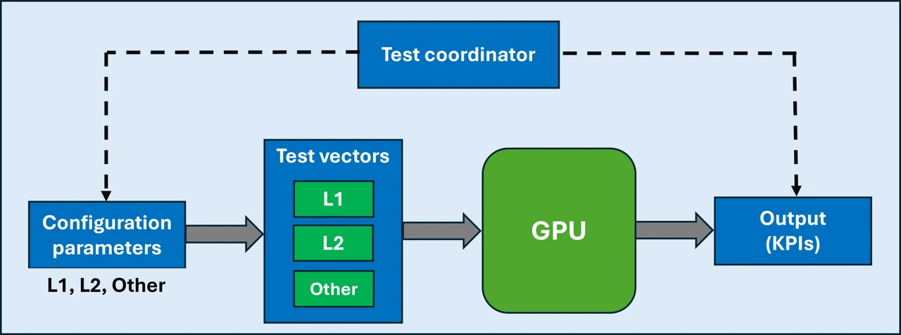
Figure 1: RANPerf benchmarking procedure

Inputs and Outputs#

Overview#

The core of RANPerf testbench is a C++ platform testbench (residing in the cubb_gpu_test_bench subfolder of the aerial_sdk/testBenches folder) paired with a user-friendly Python interface (perf subfolder of the aerial_sdk/testBenches folder). The C++ testbench takes command options and a YAML file as inputs. The Python interface generates those inputs automatically from higher-level arguments. The Python interface is the recommended way to run RANPerf benchmarking scenarios, see Figure 2.

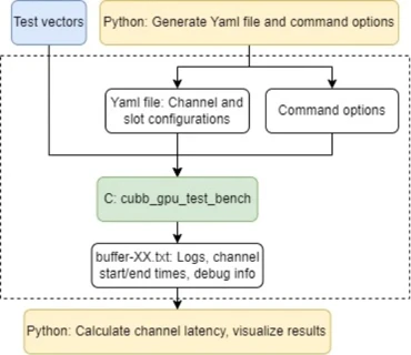
Figure 2: High-level diagram showing the use of the RANPerf testbench Python interface for generating benchmarking results

RANPerf testbench defines patterns which are a series of GPU workloads across a fixed number of slots. Figure B.1 in Appendix B shows a typical example of cuPHY (L1) processing timelines. We emphasize that:

The patterns defined for RANPerf testbench are repeatedly run on the GPU and latencies are collected across all repetitions.
In the power measurement mode, a single pattern is run --iterations times without interruption so that the GPU stays fully loaded while power is sampled.

Please refer to Appendix B (Test Case Configuration) for details on the supported configurations.

Inputs#

Test vector (TV) files of HDF5 (Hierarchical Data Format version 5) format, where one TV is provided per channel and generated by MATLAB/C++. The TVs contain channel parameters and data samples at generation time (number of PRBs, MCS, number of MIMO layers, DMRS type, etc.). In general, the cuPHY TVs are available in /mnt/cicd_tvs/develop/GPU_test_input.
YAML config file (cubb_gpu_test_config.yaml) which overrides the default TVs (override_test_vectors) by changing the Python-related configuration parameters such as the paths, GPU settings, sweep parameters, channel enable controls, timeline delays, latency budgets, etc. Note that the same HDF5 TVs can be reused across different test cases by changing only the YAML overrides, see Appendix B (Test Case Configuration) for details on the supported configurations.
Command options that can override parameters inside the YAML config file. For example, --slots 200 will override the slots: xxx value in the YAML config file.

Outputs#

JSON results file (*_sweep_graphs_avg_*.json / *_power_graphs_avg_*.json) containing:
- Configuration: Input arguments, GPU name
- Per-channel latency and on-time percentages
- Power / memory traces (power mode)
PNG plots for latency, power, memory, and temperature.
Supplementary outputs (generated by Python, consumed by the C++ testbench):
- vectors-*.yaml — per-channel slot schedule passed to the C++ testbench
- buffer-*.txt — raw console output from the C testbench
- Nsight Systems trace (.nsys-rep) when debug mode is enabled and --debug_mode nsys is used

High-Level Flow#

Load TVs for each channel – PRACH, PDCCH, CSI-RS, PUCCH, SSB, PDSCH, PUSCH, SRS, cuMAC.
Partition GPU SM resources to create multiple MPS (Multi-Process Service) contexts or Green Contexts — one context per channel or one context for multiple channels. See Section 6 for more details about the two GPU resource partitioning mechanisms. SM provisioning is an important step for performance improvement. Generally, data channels require more SMs than control channels since they are computationally more intensive, see Appendix C (SM Tuning Example) for an example describing the process of selecting SM allocations that can maximize benchmarking performance.
Sweep cell count from --start to --cap with step size --step_size, running --slots slots (--slots / nSlotPerPattern repetitions) per cell count.
Report the maximum cell count where all channels are 100% on-time – this is defined as the cell capacity.
At the confirmed cell capacity, measure steady-state GPU power, memory, and temperature.
Optionally capture Nsight Systems traces at the confirmed cell capacity.

GPU Context Modes: MPS and Green Contexts#

RANPerf testbench supports two GPU resource partitioning mechanisms: MPS and Green Contexts. In the following, the main characteristics of the two modes are described and compared against each other.

MPS#

Each channel type gets its own MPS sub-context. The --M value sets an upper bound on the number of SMs that a sub-context may use. With the used MPS dynamic partitioning, an MPS context can use any number of SMs, up to a specified upper bound; there is no static assignment of SMs to an MPS context. In this way, higher overall GPU utilization is achieved.
The Python interface automatically initiates the MPS server. If you would like to run the C++ testbench natively, start MPS manually before launching. Make sure MPS is running on the correct GPU (specify with -g <GPU_ID> or CUDA_VISIBLE_DEVICES).
MPS crash behavior:
- Possible errors include CUDA_ERROR_MPS_SERVER_NOT_READY or CUDA_ERROR_MPS_MAX_CONNECTIONS_REACHED (if the client/context limit is exhausted). In most cases a container restart is not required.
- First, try restarting MPS:
```
echo quit | nvidia-cuda-mps-control
nvidia-cuda-mps-control -d
```
- If restarting MPS does not solve the issue, restart the container as a fallback.

Green Contexts#

Green Contexts are supported for CUDA 12.4+ versions (-n flag).
Each channel type gets its own Green Context backed by a fixed subset of SMs carved out of the GPU via cuDevSmResourceSplitByCount.
Enable Green Contexts via YAML flags:
- use_green_contexts: true: Use green contexts instead of MPS
- enable_mps_for_green_contexts: false: Keep MPS running alongside green contexts (not common)

Per-Channel Context Mapping#

Each channel runs in a sub-context. Two flags control each channel independently: an enable flag (whether the channel is enabled) and an isolate flag (whether the channel gets its own dedicated sub-context or it is shared with another channel).
The SM allocation (--target / --M) lists one SM value per active isolated sub-context, in the following order:
- PRACH (if isolated)
- PDCCH (if isolated)
- PUCCH (if isolated)
- PDSCH (if isolated)
- PUSCH (if isolated)
- SSB (if isolated)
- SRS (if isolated)
- MAC (if enabled)
In the MPS mode, the SM allocation order in --target / --M matches the active isolated sub-contexts only. Please find below an example:
- When PRACH, PDCCH, and PUCCH are all isolated — target: ["8", "8", "10", "46", "66"] maps to PRACH=8 SMs, PDCCH=8 SMs, PUCCH=10 SMs, PDSCH=46 SMs, and PUSCH=66 SMs. The full GPU SM count is logically available to each context; use --M to set heterogeneous per-context limits. The list of all elements in --M may sum to more than the total GPU SMs although in practice the total number of SMs cannot be exceeded during execution.
In the Green Context mode, the SMs can be configured by the YAML config input in Python files or using the default heuristic in cubb_gpu_test_bench.cpp based on the number of SMs given in --target / --M. It is recommended to use the YAML config file for SM allocation.

MPS vs. Green Context Comparison#

This table summarizes the main characteristics of the MPS and Green Context GPU context modes:

Aspect	MPS	Green Context
CUDA version	Any version supported by Aerial	Min. CUDA Version 12.4
Requires MPS daemon	Yes	No
SM partitioning model	Upper bound; any SMs can be used	Fixed subset of SMs per sub-context
Process model	Multi-process client model	Single-process with multiple Green Contexts
Enable flag	Default mode when `use_green_contexts` is false	Enabled via `use_green_contexts: true` in YAML (equivalently `-n` in C++ testbench)
Default mode	Yes	No (use in experimental mode when better SM isolation is required)

As shown in the MPS vs. Green Context comparison table, MPS is the default GPU context mode used by RANPerf testbench.

Channel Enable and Detection#

Channel presence is communicated to the C++ testbench in two ways depending on the channel:

PDSCH and PUSCH: Always enabled by default; Python passes explicit --D / --U flags to the C++ testbench. These can be suppressed by using --no_pdsch / --no_pusch.
All other channels: Python writes the channel’s TV entries into the format vectors-XX.yaml when enabled. The C++ testbench detects those channels from the YAML content; no separate enable flag is needed.

This table summarizes the YAML key, the Python CLI, and the C++ flag/detection per channel:

Channel	YAML key	Python CLI	C++ flag/detection	Notes
PRACH	`prach: true`	`--prach`	Present in `vectors-XX.yaml`	Optional channel; enabled when test vectors are present
PDCCH	`pdcch: true`	`--pdcch`	Present in `vectors-XX.yaml`	Optional channel; often used with CSI-RS and SSB
CSI-RS	`csirs: true`	`--csirs`	Present in `vectors-XX.yaml`	Optional; always co-located with PDCCH in timelines
PUCCH	`pucch: true`	`--pucch`	Present in `vectors-XX.yaml`	Optional uplink control channel
SSB	`ssb: true`	`--ssb`	Present in `vectors-XX.yaml`	Optional; typically paired with PDCCH and CSI-RS
PDSCH	`no_pdsch: true` (to disable)	`--no_pdsch` / implicit `--D`	`--D` flag when enabled	Enabled by default; Python passes `--D` unless `no_pdsch: true` is set
PUSCH	`no_pusch: true` (to disable)	`--no_pusch` / implicit `--U`	`--U` flag when enabled	Enabled by default; Python passes `--U` unless `no_pusch: true` is set
SRS (enabled with DLBFW and ULBFW by default)	`rec_bf: true`	`--rec_bf`	Present in `vectors-XX.yaml`	SRS and BFW generation workloads cannot be enabled independently
cuMAC	`mac: true`	`--mac` (Python also passes `--T`)	`--T` flag when enabled	Python passes `--T` when `mac: true` is set

Channel Isolation and Sub-Contexts#

Channel isolation controls whether a channel gets its own sub-context or shares one. The C++ isolation flags (--P, --Q, --X, --Z, --B) are passed by Python only when the channel is both enabled and isolated. If a channel is enabled but not isolated, it shares another channel’s sub-context and no isolation flag is sent to C++.

This table summarizes the YAML key, the Python CLI, and the C++ flag per channel.

Channel	YAML key	Python CLI	C++ flag	Notes
PRACH	`prach_isolate: true`	`--prach_isolate`	`--P`	Shares PUSCH sub-context when not isolated
PDCCH	`pdcch_isolate: true`	`--pdcch_isolate`	`--Q`	Shares PDSCH sub-context when not isolated
PUCCH	`pucch_isolate: true`	`--pucch_isolate`	`--X`	Shares PUSCH sub-context when not isolated
SSB	`ssb_isolate: true`	`--ssb_isolate`	`--B`	Shares PDCCH sub-context when not isolated
SRS	`srs_isolate: true` (valid when `rec_bf: true`)	`--srs_isolate`	`--Z`	Shares PUSCH sub-context when not isolated
PDSCH (DLBFW if exists)	None	Implicit when enabled	`--D`	Always owns its own sub-context
PUSCH (ULBFW if exists)	None	Implicit when enabled	`--U`	Always owns its own sub-context
cuMAC	None	`--mac`	`--T`	Always dedicated when enabled

UL/DL Scheduling Modes#

The -u flag selects the UL/DL slot scheduling mode. Note that only -u 5 with the 10-slot TDD pattern DDDSUUDDDD is extensively used in practical system deployments; other modes are currently experimental but may be added in the future as necessary.

This table summarizes the functionality of the supported UL/DL scheduling mode:

Mode	Description
`-u 5`	Slot pattern DDDSUUDDDD; supports 10-slot and legacy 8-slot variants; it also supports per-channel context flags, i.e., `--P` for PRACH, `--Q` for PDCCH, `--X` for PUCCH, and cuMAC contexts

Cell Aggregation and Capacity Sweep#

Cell Aggregation Modes#

Each channel can either create a separate pipeline object for each of its test vectors or perform cell aggregation — grouping all test vectors in a slot into a single pipeline object. Cell aggregation reduces kernel launch overhead and is recommended for enabling lower latency. Note that beamforming-only workloads and SRS do not currently support cell aggregation flags.

This table summarizes the different cell aggregation modes per channel:

Channel/Flag	YAML/CLI key	Behavior
PDSCH (default)	None	One PDSCH pipeline object per test vector per slot; the number of objects is equal to the number of PDSCH cells per slot
PDSCH aggregation	`--g` / `groups_dl: true`	One PDSCH pipeline object executes all PDSCH test vectors in a slot by stitching multiple cells together; it is the recommended option
PUSCH (default)	None	One PUSCH pipeline object per test vector per slot; each cuPHY PUSCH test vector is for a single cell
PUSCH aggregation	`--g` / `groups_pusch: true`	Enables PUSCH cell aggregation; it is the recommended option.
PDCCH (default)	None	One PDCCH pipeline object per test vector per slot
PDCCH aggregation	`--g` / `groups_dl: true`	One PDCCH pipeline object executes all PDCCH test vectors in a slot; note that it uses the same grouping flag as PDSCH
SSB (default)	None	One SSB pipeline object per test vector per slot
SSB aggregation	`--g` / `groups_dl: true`	One SSB pipeline object executes all SSB test vectors in a slot; note that it uses the same grouping flag as PDSCH
CSI-RS (default)	None	One CSI-RS pipeline object per test vector per slot
CSI-RS aggregation	`--g` / `groups_dl: true`	One CSI-RS pipeline object executes all CSI-RS test vectors in a slot; a single kernel per component is used even if `-b` is not set.
PRACH (default)	None	One PRACH pipeline object per test vector per slot; each cuPHY PRACH test vector contains a cell group with a single cell
PRACH aggregation	`--g` / `groups_pusch: true`	Enables PRACH cell aggregation; note that it uses the same grouping flag as PUSCH

Capacity Sweep#

RANPerf testbench sweeps the cell count from --start up to --cap, running --slots slot repetitions per count. It reports per-channel latency statistics as well as the maximum cell count where all channels meet their deadlines 100% on-time. When --step_size is used, it sweeps the following counts: {start, start+step_size, start+step_size*2, ..., cap}. The Python interface will print out the cell capacity or a warning — if no cell count passes or if the max cell count passes.

Option fix_ul_cell_count = N fixes UL processing at N cells regardless of the DL sweep count — this allows decoupling of UL and DL scaling and allows the DL to sweep beyond the UL operating point.

Streams and CUDA Graphs#

One slot of each channel is processed sequentially across all cells. The GPU scheduler overlaps workloads from different contexts spatially – across different SM partitions – and temporally – UL decode / DL encode pipelines overlap across slots.

The Stream mode (-m 0) uses standard CUDA streams and is the default option.

In the Graph mode (-m 1), a CUDA graph per pipeline object is created and updated/replayed across each slot — this yields lower latency and lower CPU overhead. The Graph mode is the recommended option for capacity measurement.

Note that cuMAC currently supports only the Stream mode.

This table summarizes the functionality of each mode:

Flag/Mode	Description
`-m 0`	Stream mode (default); it is used to generate power and trace runs where the accuracy of the measured minimum latency is less critical
`-m 1`	Graph mode; it is used for achieving lower latency, and it is the recommended mode for measuring the cell capacity

Reference Checks#

Reference checks validate the GPU outputs against reference TVs from cuPHY. For the Python interface, --ref_check enables reference checks for all channels and produces the command options listed in the following table for the C++ testbench. The --c interface is the recommended option; for example, set: --c PDSCH,PUSCH,PUCCH for enabling reference checks for PDSCH, PUSCH, and PUCCH.

Warning

Enabling reference checks significantly increases workload latency due to the required CPU–GPU data comparisons and, thus, the results will not reflect real-time performance. Therefore, the user should not use reference checks in cell capacity or latency measurements.

This table lists the reference check command options for the C++ testbench:

Command option (flag)	Channel(s)	Behavior
`-k`	PDSCH	Enables PDSCH reference check; terminates on mismatch with reference TVs
`--k`	PDCCH	Enables PDCCH reference check; terminates on mismatch with reference TVs
`-b`	PUSCH	Enables PUSCH reference check; terminates on mismatch with reference TVs
`--c <ch1, ... chN>`	Any subset of PUSCH, PDSCH, PDCCH, PUCCH, PRACH, SSB, CSI-RS, SRS	Unified interface; enables reference check for each of the listed channels and terminates on mismatch with reference TVs per channel

Scaling to Larger Cell Counts#

The default branch always supports a specific worst-case configuration in terms of the maximum number of cells that can be scheduled in a single cell group. These worst-case configurations are determined by macros in cuphy.h and are used to place upper bounds on GPU memory allocations for the various cuPHY channels.

For any multi-cell experiment where the user would like to scale the number of cells beyond what is currently supported, the user needs to modify the values of the parameters. The following table demonstrates how the parameters of each channel should be modified and how the limits should be calculated. Note that PUCCH Fx, where x is 0, 1, 2, or 3, in Table 8 refers to the different PUCCH formats.

This table summarizes how to modify the channel parameters for scaling to larger cell counts:

cuPHY channel	Parameter	Current value	How to calculate the new value	Comment
PDSCH	`PDSCH_MAX_UES_PER_CELL_GROUP`	128	Number of UEs per cell × number of cells	Assumes homogeneous cells. If not, pick the worst-case number of UEs for your cells and multiply by the number of cells, or use the total number of UEs for your cell group.
	`PDSCH_MAX_UE_GROUPS_PER_CELL_GROUP`	128	Number of UE groups per cell × number of cells	Same as above but for UE groups
	`PDSCH_MAX_CELLS_PER_CELL_GROUP`	64	Number of cells	Usually a much lower max limit is passed as part of static parameters and used in GPU allocations for both cuPHY and cuBB tests
	`PDSCH_MAX_HET_LDPC_CONFIGS_SUPPORTED`	64	See comment	Maximum number of heterogeneous LDPC encoder configurations in a cell group (across all cells) in PDSCH. A distinct LDPC configuration is determined by {BG (base graph), Zc (lifting size), F (filler bits), number of code blocks}
	`PDSCH_MAX_UES_PER_CELL`	64	Number of UEs per cell	Not currently used unless the code is modified to fall back to the old single-cell-in-a-cell-group limit
SRS	`CUPHY_SRS_MAX_N_USERS`	192	Number of SRS UEs	Set based on total SRS UEs across cells
	`MAX_N_SRS_CELL`	24	Number of cells	Set to the maximum number of SRS cells in the scenario
PUSCH	`MAX_N_TBS_PER_CELL_GROUP_SUPPORTED`	128	Number of UEs (transport blocks) per cell group	Use number of UEs per cell group
	`MAX_N_USER_GROUPS_SUPPORTED`	128	Number of UE groups per cell group	Can be set equal to `MAX_N_TBS_PER_CELL_GROUP_SUPPORTED`
PUCCH F0	`CUPHY_PUCCH_F0_MAX_GRPS`	160	Number of UCI groups per cell × number of cells	If exceeded, additional UCIs/UCI groups are dropped and warnings are printed
PUCCH F1	`CUPHY_PUCCH_F1_MAX_GRPS`	384	Number of UCI groups per cell × number of cells	Peak cell patterns use up to 24 UCI groups per cell (one UCI per group). If exceeded, no more UCI groups are scheduled and warnings are printed
PUCCH F2	`CUPHY_PUCCH_F2_MAX_GRPS`	256	Total number of UCIs	If exceeded, additional UCIs/UCI groups are dropped and warnings are printed
PUCCH F3	`CUPHY_PUCCH_F3_MAX_GRPS`	512	Total number of UCIs	If exceeded, additional UCIs/UCI groups are dropped and warnings are printed

Warning

If the user does not modify the values of the parameters in the table above before running a higher cell count, errors such as the following one may be encountered:

Error! nPdschCellsPerStrm (some value) > PDSCH_MAX_CELLS_PER_CELL_GROUP 1.
Update the max. limit in the header file.

Warning

The user should not push changes to the values of the parameters in the table above on the default branch if they are solely used for experiments as they can have performance/capacity cell implications, e.g., impact on the size of GPU memory allocations, memory size and duration, etc.

Note

The Build flag ENABLE_64C=ON modifies the macros in cuphy.h to enable testing for higher cell counts. See the following section (How to run L1 GPU benchmarking tests) for the full build command.

How to Run Benchmarking Tests on RANPerf Testbench#

Prerequisites#

A Linux server with a supported NVIDIA GPU.
Access to Aerial SDK repository at NVIDIA/aerial-cuda-accelerated-ran
Sample YAML configuration files are available, see details in Appendix B (Test Case Configuration).
TVs of HDF5 format corresponding to the YAML files. Note that the path to the HDF5 TVs must match the testvectors_folder inside the YAML configuration files.

Build Testbench for RANPerf Benchmarking#

Checkout the Aerial SDK:
- The open-source repository sits at: github.com/NVIDIA/aerial-cuda-accelerated-ran
- Follow the README.md file to clone the Aerial repository:
```
git clone --recurse-submodules https://github.com/NVIDIA/aerial-cuda-accelerated-ran.git
cd aerial-cuda-accelerated-ran
```
- Enable git LFS and pull files:
```
sudo apt install git-lfs
git lfs pull
```
- Note the related code bases:
  - C++ test bench: testBenches/cubb_gpu_test_bench/
  - Python interface: testBenches/perf/
    - Config Template: testBenches/perf/cubb_gpu_test_config.yaml
  - 5G Model for TV generation: 5GModel/nr_matlab
Start the Aerial container:
- ./cuPHY-CP/container/run_aerial.sh
- If the system does not have gdrcopy, you can try to bypass the gdrcopy check since it is not used in L1 GPU benchmarking:
```
AERIAL_CHECK_GDRDRV=0 cuPHY-CP/container/run_aerial.sh
```
- The default container name is c_aerial_${USER}. The host path aerial_sdk will be mapped to /opt/nvidia/cuBB inside the container.
- Notes:
  - If you encounter permission access issues, login to the docker using your username and GitLab personal access token. After login succeeded, you may need to logout the remote session and login again.
  - Optionally you can modify the run_aerial.sh script to add any path mapping (like personal NFS) by -v <host_path>:<container_path> \, and run in detached mode (docker run -d --platform …).
  - To use an existing container, you can also use cuPHY-CP/container/attach_aerial.sh or docker exec xxx.
Build inside the Aerial docker container:
- Default build command:
```
cd /opt/nvidia/cuBB
bash testBenches/phase4_test_scripts/build_aerial_sdk.sh \
  --targets cubb_gpu_test_bench
```
- Example of customized build options:
```
cd /opt/nvidia/cuBB
bash testBenches/phase4_test_scripts/build_aerial_sdk.sh \
  --targets cubb_gpu_test_bench \
  --cuda-archs 80-real 90-real 100-real 120-real \
  -- -DCMAKE_BUILD_TYPE=Release -DENABLE_CUMAC=OFF -DENABLE_64C=ON
```
- Notes:
  - ENABLE_CUMAC=OFF means no cuMAC in the testbench (using --mac will cause an error in this case); ENABLE_64C=ON modifies the macros in cuphy.h to enable testing for higher cell counts.
  - The build produces: $cuBB_SDK/build.$(arch)/testBenches/cubb_gpu_test_bench/cubb_gpu_test_bench
  - Here build.$(arch) can be build.aarch64 or build.x86_64

Test Workflow#

It is assumed that tests are run in the testBenches/perf folder inside the container.

Basic test:

The basic test is a cell capacity and power benchmark with given YAML config (timeline, SM allocation, GPU power, GPU frequency).

C++ functionality test:

The goal of this test is to obtain ref_check PASS, which ensures that the TVs and the testbench process the data correctly.

The user should run:

python3 measure.py --yaml <Yaml config> --start 2 --cap 2 --enable_ref_check

Example output for PASS:

Number of active cells: 2+0(8,8,64,50,60)
[ref_check 2 cells] PASS (PDSCH: PASS, PUSCH: PASS, PRACH: PASS, PDCCH: PASS, CSIRS: PASS, PUCCH: PASS)
enable_ref_check is on, skip cell capacity check
-> [ref_check 2 cells] PASS

Cell capacity test:
- The goal is to measure the cell capacity, which is the maximum number of cells that are 100% on-time (all slots of each channel’s workload are completed within its configured latency budget).
- The user should run:
```
python3 measure.py --yaml <Yaml config> --start X --cap Y --slots T
```
- This command will run the test for X, X+1, X+2, …, Y cells, each for T slots. There can be four outcomes:
  - The measured cell capacity is {cellCapacity} based on T slots run (100% on-time for all channels)
  - No cell pass:
    Warning: no cell count passed based on {sweeps['testConfig']['sweeps']} slots run, unknown cell capacity (100% on-time for all channels), please try smaller cell counts.
    This means even the lowest cell count X failed; try decreasing X and Y.
  - Max cell pass:
    Warning: max cell count {maxCellTested} passed based on {sweeps['testConfig']['sweeps']} slots run, unknown cell capacity (100% on-time for all channels), please try larger cell counts.
    This means even the highest cell count Y passed; try increasing X and Y.
  - No successful run:
    Warning: no successful run is completed, unknown cell capacity (100% on-time for all channels), please retry
    This means none of the cells in [X, Y] runs successfully. Need further debug.
- Note:
  - The latency test mode will perform the sequence “setup → run one pattern → setup → run one pattern → setup …”, which is time-consuming. Therefore, it is recommended to use a smaller number of slots, e.g., 30, with a wider {X, Y} range to identify a narrower {X, Y} range for running the test with a larger number of slots, e.g., 300 slots, to measure the cell capacity.
- After the latency test, there will be a json file <sm_alloc_str>_sweep_graphs_avg_F08.json that has the test config and the latency results. To get the CDF plot from the latency tests, run the following for all cells [X, Y]:
```
python3 compare.py --filename <sm_alloc_str>_sweep_graphs_avg_F08.json
```
- or run for a selected number of cells (say n1 and n2)
```
python3 compare.py --filename <sm_alloc_str>_sweep_graphs_avg_F08.json <sm_alloc_str>_sweep_graphs_avg_F08.json --cells n1+0 n2+0
```
- A compare-<date>.png file will be generated. Please make sure that the number of --filenames match with --cells. Other options are:
  - --short_legend: generates shortened legends in the CDF plots
  - --filenames, same as --filename
Power measurement test:
- It is assumed that cell capacity is N based on the measurement from the Cell capacity test, see above.
- To measure the GPU power, run:
```
python3 measure.py --yaml <Yaml config> --start N --cap N --slots 10 --iterations 2000 --delay 0 --measure_power
```
- This will run the test pattern for N cells and 2000 iterations without any delay between patterns (setup once and run multiple times). This will also run nvidia-smi in a dedicated thread to measure the GPU status while the tests are running.
- The power test mode will perform “setup → run --iterations pattern”, which should be faster than the latency mode. Note that the test will draw significant power and increase the GPU temperature substantially.
- After the power test, there will be a json file <sm_alloc_str>_power_graphs_avg_F08.json. To obtain the power/memory/temperature, run:
```
python3 power.py --filenames <sm_alloc_str>_power_graphs_avg_F08.json --cells N+0
python3 memory_plot.py --filenames <sm_alloc_str>_power_graphs_avg_F08.json --cells N+0
python3 temperature_plot.py --filenames <sm_alloc_str>_power_graphs_avg_F08.json --cells N+0
```
- The following info will be provided on the command window.
```
Maximum power: xxxx, Frequency std.: xxxx
Maximum memory used: xxxx MB, Memory frequency std.: xxxx
Minimum temperature: xxxx, Maximum temperature: xxxx
```
Optional Nsys trace capture:
- The goal is to capture an Nsys trace for further analysis. The key change is to use --debug --debug_mode nsys. It is recommended to add --enable_nvprof to skip the setup stage. Since Nsys capture is time-consuming, it is recommended to use a small number of slots, e.g., 10 or 20 slots, or a small number of iterations.
- To capture an Nsys trace in the latency measurement mode, run
```
python3 measure.py --yaml <Yaml config> --start X --cap Y --slots 10 --debug --debug_mode nsys --enable_nvprof
```
- To capture an Nsys trace in the power measurement mode, run
```
python3 measure.py --yaml <Yaml config> --start N --cap N --slots 10 --iterations 100 --delay 0 --measure_power --debug --debug_mode nsys --enable_nvprof
```
- This will generate a time-stamped nsys-rep file.
Test artifacts:
- The most important test results are the json files, png figures, and nsys report. It is recommended to save those along with the yaml configuration file.
- Additionally, vectors-*.yaml and buffer-*.txt are the raw input to and output from the C++ testbench, respectively, which provide additional test details.

Test with different GPU power and frequency:

For tests using different GPU power, use --power <power_cap>; note that nvidia-smi -pl <power_cap> will be executed before running the test.
For tests using different GPU clock frequency, use --freq <clock_freq>; note that nvidia-smi -lgc <clock_freq> will be executed before running the test.
In general, the user should use the following command for more flexible benchmarking tests without generating many YAML configuration files:
```
python3 measure.py --yaml <Yaml config> --freq <clock_freq> --power <power_cap> --start X --cap Y --slots T
```

Test with different SM allocations:

The specific SM allocation plays an important role in L1 GPU benchmarking. To test a customized SM allocation in the test, add --target <sm_alloc>, e.g., --target '["8", "8", "10", "46", "66"]', in all the above test commands.
If an SM allocation does not match the channel isolation strategy, an error will be generated. Note that the specific SM allocation will also impact the json file naming.
Please refer to Appendix C (SM Tuning Example) for more details.

Test with given GPU power, flexible GPU frequency:

In this test, we have a fixed GPU power budget and only the GPU clock frequency can vary. Therefore, the user will need to run a range of frequencies, measure the cell capacity and power, and compare the result with the fixed GPU power budget to obtain the final result. This step can be very time-consuming.
A more efficient method is to start with the power measurement, sweep over a wide range of frequencies and cell counts. Since the power measurement is much faster, the said sweep can take place rather quickly. Then, the user can identify the <freq, cell count> pair that meets the GPU power budget (or is very close to the power budget) and run the latency test for the selected <freq, cell count> pair. This method will reduce the number of latency tests, which is key to reducing the overall test time.

Troubleshooting#

If error CUDA_ERROR_MPS_MAX_CONNECTIONS_REACHED or error no CUDA-compatible device are detected is encountered, try restarting the container by running docker restart c_aerial_${USER}.
As the Aerial container does not include matplotlib by default, run pip install matplotlib before plotting the latency CDFs or the GPU traces.

Quick Start#

Figure 3 summarizes the steps to prepare (Step 1), build (Step 2), run (Step 3), and generate outputs (Step 4) of RANPerf benchmarking. Figure 3 can be used as a Quick Start guide.

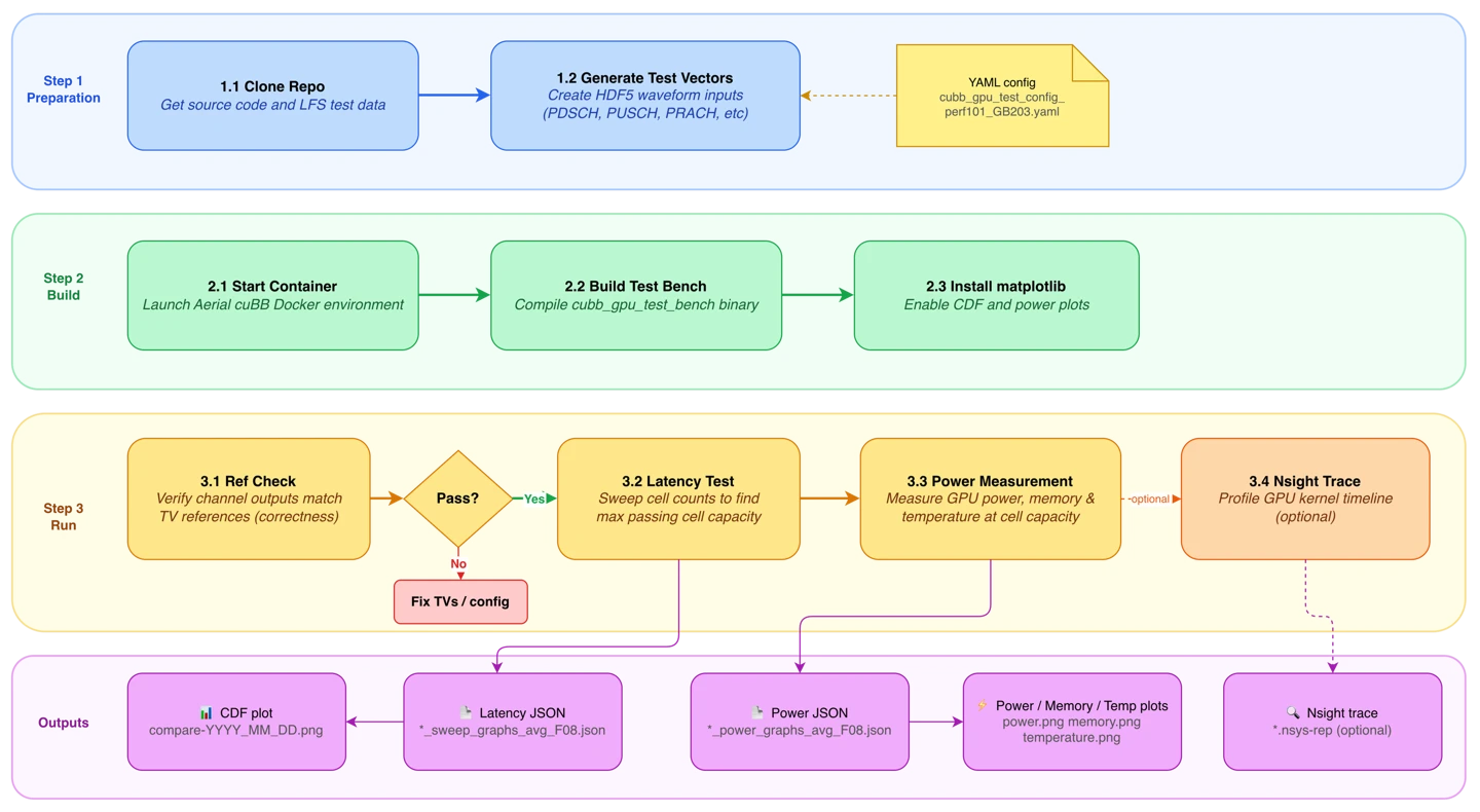
Figure 3: Summary of RANPerf benchmarking steps that can be used as a Quick Start guide

Appendices#

Appendix A: Glossary#

CDF: Refers to Cumulative Distribution Function plots. These plots visualize test statistics and can be generated using matplotlib to analyze performance metrics across different system configurations.
CLI (Command-Line Interface): Refers to interacting with AI systems by typing text-based commands into a terminal rather than clicking buttons in a graphical user interface (GUI).
CUDA (Compute Unified Device Architecture): A parallel computing platform and programming model. It enables developers to utilize NVIDIA GPUs for general-purpose computing by providing a software layer that interacts with the hardware. The ecosystem includes a comprehensive toolkit, libraries, and APIs designed to accelerate applications across various domains, such as AI and data science. It supports multiple programming languages, including C++ and Python, and features specialized components for safety-critical environments and multinode configurations.
cuPHY: NVIDIA GPU-accelerated L1 (PHY) library for 5G NR used by Aerial.
cuMAC: NVIDIA GPU-accelerated L2 (MAC) scheduler library for 5G NR used by Aerial.
DL: Downlink or link between base station (BS) and user equipment (UE).
Early Hybrid Automatic Repeat reQuest (Early HARQ or E-HARQ): An advanced feedback optimization technique for 5G which predicts whether a receiver will successfully decode a packet before the full channel-decoding or transmission cycle finishes, leading to a reduction of over-the-air feedback latency.
Green Context: CUDA feature (from 12.4) that creates GPU contexts backed by fixed SM subsets, providing isolation between workloads.
KPIs (Key Performance Indicators): Main performance metrics to evaluate performance; in the context of RANPerf testbench, the KPIs are cell capacity, latency, GPU power, GPU memory, and GPU temperature.
MCS (Modulation and Coding Scheme): An operational index that dynamically determines how data is formatted for transmission over the air interface. An MCS index maps directly to a specific combination of two fundamental digital communication techniques: Modulation order (Qm) that determines how many bits of digital data are packed into a single radio resource element (known as a modulation symbol) and the code rate (R) that represents the ratio of useful information bits to the total transmitted bits (which include redundant parity bits added for Low-Density Parity-Check (LDPC) error correction).
MPS (Multi-Process Service): NVIDIA mechanism that allows multiple CUDA processes to share a GPU concurrently with soft SM partitioning. See https://docs.nvidia.com/deploy/mps/latest/index.html for a detailed explanation of the service.
Network File System (NFS): A networking protocol for distributed file sharing. It allows users to store and retrieve data across networks as if it were on local storage. Originally developed by Sun Microsystems in 1984, it uses Remote Procedure Calls (RPCs) to route requests between clients and servers. Administrators can share portions of a file system, enabling authorized clients to mount these shares. NFS requires close-to-open cache coherency to ensure data.
On-time: Percentage of slots where a channel’s workload completes within its configured latency budget; 100% on-time across channels defines cell capacity in RANPerf L1 benchmarking.
Pattern: A fixed slot-level schedule of channel workloads (DL/UL, control/data) used repeatedly by RANPerf testbench for capacity and power measurements.
PRB (Physical Resource Block): The fundamental unit of radio resources in 5G consisting of 12 REs (Resource Elements of subcarriers) in the frequency domain and a single time slot in the time domain.
TV (Test Vector): Pre-generated input/output dataset (often in HDF5 format) describing waveform parameters and reference results for each channel and cell.
UL: Uplink or link between UE and BS.

Appendix B: Test Case Configuration#

Introduction#

The test is driven by a single YAML file passed to measure.py:

cd $cuBB_SDK/testBenches/perf
python3 measure.py --yaml cubb_gpu_test_config.yaml

The base template is testBenches/perf/cubb_gpu_test_config.yaml. Keys under config: map directly to measure.py / measure/cli.py CLI flags (without the leading --). CLI flags override YAML values if both are provided. Three sections – start_delay, override_test_vectors, and latency_budget – are YAML-only and are written into the generated files of format vectors-XX.yaml or used by the Python capacity-check logic.

For example, the user could run a 200-slot test for GPU clock frequency of 1610 MHz (regardless of what is defined inside the YAML file) by

cd $cuBB_SDK/testBenches/perf
python3 measure.py --yaml cubb_gpu_test_config.yaml --slots 200 --freq 1610

Config#

Paths and Inputs

This table provides the description and examples for config paths and inputs:

Key	Description	Example
`usecase`	Test use case ID; F08, F09, and F14 supported	F08 supported; F09 and F14 are reserved for future configurations
`testbench_folder`	Path to the built `cubb_gpu_test_bench` folder (`--cuphy`)	`/opt/nvidia/cuBB/build.aarch64/testBenches` or `/opt/nvidia/cuBB/build.x86-64/testBenches`
`testvectors_folder`	Root directory for HDF5 TV files (`--vector_folder`)	`/opt/nvidia/cuBB/testVectors`
`vector_files`	Per-channel list of HDF5 TV filenames. See text after Table B.1 for details.

vector_files — each key is a channel name; each value is a list of HDF5 filenames.
For cuPHY, each TV is only for a single cell and single channel. In L1 GPU benchmarking tests, TV selection is round robin-based: tv_idx = cell_idx % len(list). In most cases, one cuPHY TV per channel is sufficient, and all cells will use the same TV for all slots.
- All 5GModel TVs are saved in NFS, which can be found in /mnt/cicd_tvs/develop/GPU_test_input. These TVs are updated daily by CICD.
- Alternatively, TVs can be manually generated by testCompGenTV_xxx.m from 5GModel where xxx can be any PHY channel, ulmix, or dlmix.
- If /mnt/cicd_tvs/ is not mounted, the user can manually mount it by running:
```
sudo mount -t nfs hp-5g.dyn.nvidia.com:/srv/nfs4/cicd/cicd-tvs /mnt/cicd_tvs
```
Examples of cuPHY vector_files for different channels are listed below:
- PDSCH: TVnr_DLMIX_9905_PDSCH_gNB_CUPHY_s0p5.h5, TVnr_DLMIX_9906_PDSCH_gNB_CUPHY_s0p5.h5
- PUSCH: TVnr_ULMIX_4548_PUSCH_gNB_CUPHY_s0p5.h5
- PRACH: TVnr_ULMIX_4544_PRACH_gNB_CUPHY_s0p3.h5
- PDCCH: TVnr_DLMIX_9696_PDCCH_gNB_CUPHY_s0p1.h5
- PUCCH: TVnr_ULMIX_4566_PUCCH_F1_gNB_CUPHY_s0p18.h5
- SSB: TVnr_DLMIX_9481_SSB_gNB_CUPHY_s0p1.h5
- CSIRS: TVnr_DLMIX_10047_CSIRS_gNB_CUPHY_s0p2.h5

If you encounter the following error, it is most likely a TV issue. Please try pulling the latest aerial_sdk changes and using the latest TVs.

terminate called after throwing an instance of 'cuphy::cuphyHDF5_exception'
what(): No such scalar or structure field with the given name exists

GPU controls

This table provides the description and examples of config GPU controls:

Key	Description	Example
`gpu`	GPU device index (`--gpu`)	0
`freq`	Target GPU clock frequency in MHz (`--freq`)	1610
`power`	GPU power limit in W (`--power`)	165
`target`	SM allocation per active isolated sub-context. The channel order is: PRACH, PDCCH, PUCCH, PDSCH, PUSCH, SSB, SRS.	`["8", "8", "10", "46", "66"]`

Note

In testBenches/perf/measure.py, the script first checks the current GPU clock frequency, power limit, and persistence mode, and saves those settings. It then attempts to enable the persistence mode and update the GPU clock frequency and power limit only if they differ from the values specified in the YAML configuration file. After the test completes, the script restores the GPU settings to their original values. All those steps can be handled automatically, and nvidia-smi is used in those steps.

TDD priorities

The TDD priorities are listed in the following table. As usual, the smaller number the higher the priority. In the current setup, DL channels/functions have higher priority than the UL ones.

This table lists the TDD priorities:

Channel/function	Priority level
PUSCH	3
PUSCH2	3
ULBFW	3
PUCCH	2
PUCCH2	2
PRACH	2
UL_ORDER	0
UL_SRS_ORDER	0
SRS	3
PDSCH	1
DLBFW	2
PDCCH	1
CSI-RS	1
SSB	1
GPU_CMN	0

Sweep settings and duration

This table lists the TDD patterns and TDD slot configuration:

Key

Description

tdd_pattern

dddsuudddd (10-slot pattern, most-used case)

tdd_slot_config

Specify which slot has DL or MAC workload. Each array is a per-slot traffic activity mask for the TDD slot pattern: If the value is 1, this means that the corresponding channel carries traffic in this slot and TVs are generated; if the value is 0, the channel is idle in this slot (no traffic scheduled). Note that the array length must be equal to the number of slots per pattern (see example below).

Please find below an example slot configuration of different channels/workloads for the 10-slot TDD pattern dddsuudddd:

PDSCH: [0, 0, 1, 1, 1, 1, 1, 1, 1, 0]
PDCCH: [0, 0, 1, 1, 1, 1, 1, 1, 1, 0]
CSIRS: [0, 0, 1, 1, 1, 1, 1, 1, 1, 0]
PBCH: [0, 0, 0, 0, 0, 0, 1, 1, 1, 0]
MAC: [1, 1, 1, 1, 1, 1, 1, 1, 1, 1] (same with latency run)

Please find below a list of sweep parameters with example values:

start: Minimum cell count to sweep, e.g., 16 (typically using the confirmed cell capacity N)
cap: Maximum cell count to sweep, e.g., 18 (typically using the confirmed cell capacity N)
step_size: Cell count increment per sweep step, e.g., 1
iterations: Average number of iterations per sweep point, e.g., 2000
slots: Slot repetitions per pattern per iteration, must be a multiple of pattern length, e.g., 300
delay: Delay-kernel duration in µs between pattern setup and run, e.g., 10000
For latency measurement: slots=300, iterations=1, delay=10000
For power measurement: slots=10, iterations=2000, delay=0

Feature toggles

This table lists the feature toggles:

Key	Default value	Description
`graph`	true	Use of CUDA graphs; recommended for achieving lower latency
`save_buffers`	true	Save intermediate buffers `buffer-xx.txt` where `xx` is the cell count
`test`	false	Test mode: Generates YAML/CLI only, do not run.
`measure_power`	false	Power measurement mode
`enable_ref_check`	false	Enables reference check for all workloads; do not use during latency or power runs
`use_green_contexts`	false	Use CUDA green contexts instead of MPS (as mentioned before, it needs CUDA version 12.4+)
`enable_mps_for_green_contexts`	false	Keep MPS alongside green contexts; in experimental mode
`enable_nvprof`	false	Enables profiler start/stop inside the C++ testbench to reduce the scope of trace captures
`enable_gpu_metric`	false	Adds `--gpu-metrics-device` to nsys command.
`setup_once`	false	Skips per-pattern re-setup; reuses the TVs of the first pattern to run repeatedly; good for SM tuning (see Appendix C for details on SM tuning)
`enable_sqlite`	false	Exports SQLite file in nsys
`debug`	false	Enables debug mode.
`debug_mode`	nsys	Debug mode selector: cta, incu, ncu, nsys, nsys_simple, triage; nsys is most used

Channel workload toggles and isolation

This table lists the workload toggles and isolation with default values:

Key	Default value	Description
`no_pdsch`	false	Set to true to disable PDSCH
`no_pusch`	false	Set to true to disable PUSCH
`prach`	true	Includes PRACH workload
`prach_isolate`	true	Runs PRACH in its own sub-context
`pdcch`	true	Includes PDCCH workload
`pdcch_isolate`	true	Runs PDCCH in its own sub-context
`pucch`	true	Includes PUCCH workload
`pucch_isolate`	true	Runs PUCCH in its own sub-context
`ssb`	true	Includes SSB workload
`ssb_isolate`	true	Runs SSB in its own sub-context
`csirs`	true	Includes CSI-RS workload; co-located with PDCCH
`rec_bf`	false	Enables reciprocal beamforming; note that it enables SRS, DLBFW, and ULBFW together
`srs_isolate`	false	Runs SRS in its own sub-context; note that it is only relevant when `rec_bf: true`
`mac`	false	Runs cuMAC in a dedicated sub-context.
`mac_timer`	true	cuMAC uses its internal timer
`uci_timing`	false	Enforces separate UCI-on-PUSCH latency budget
`fix_ul_cell_count`	-1	Fixes UL channels at N cells; -1 enables sweep across all cells
`fix_dl_cell_count`	-1	Fixes DL channels at N cells; -1 enables sweep across all cells

Cell grouping and packing

This table lists the cell grouping and packing options with default values:

Key	Default value	Description
`groups_dl`	true	Uses DL cell groups for PDSCH/PDCCH (recommended)
`pack_pdsch`	true	Uses packed DL cell groups for PDSCH (recommended)
`groups_pusch`	true	Uses UL cell groups for PUSCH (recommended)

PUSCH and LDPC options

This table lists the PUSCH and LDPC options with default values:

Key	Default value	Description
`ldpc_parallel`	true	Runs LDPC decoder TBs in parallel; recommended option
`pusch_cascaded`	true	Starts PUSCH2/PUCCH2 after PUSCH1 completes
`pusch_subslot_proc`	“0”	Subslot processing mode: “0” = disable, “1” = enable. Since we only support no more than 2 PUSCH workloads, the valid inputs are: “0”, “1”, “00”, “01”, “10”, “11”

cuMAC options

This table lists the cuMAC keys and their functionality with default values:

Key	Description
`modules_called`	List of 4 boolean parameters [UE selection, PRG allocation, layer selection, MCS selection]; set to 0 to disable
`cumac_light_weight_flag`	Per-slot flag values: 0 = heavy kernel, 1 = light (SRS compute), 2 = light (SRS load); configurable for up to 10 slots
`perc_sm_num_thrd_blk`	Per-slot percentage of SMs for thread blocks; configurable for up to 10 slots
`half_precision`	0 = float32, 1 = half precision.
`sch_alg`	Scheduling algorithm: 0 = Round Robin, 1 = Proportional Fair.
`hetero_ue_sel_cells`	0 = disabled, 1 = heterogeneous UE selection across cells

Overriding Test Vectors#

This functionality allows overriding TV parameters inside the HDF5 TVs at runtime, and is only supported by YAML, see the following table.

This table describes the option to override configuration parameters:

Key	Default value	Description
`enable_override`	false	Master option to enable/disable all override configs; if set to false, all parameters in this section will be ignored

In the following, the override parameter list per channel for PUSCH, PUCCH, and PDSCH is provided. The user should set any parameter to -1 in order to use the TV default value.

PUSCH overrides:

This table lists the override parameters for PUSCH:

Key	Default value	Description
`ldpc_max_num_iterations`	10	Fixed maximum number of LDPC decoder iterations
`ldpc_max_num_iterations_algorithm_index`	0	LDPC max-iteration strategy (0 = fixed, 1 = LUT, 2 = per-UE)
`open_ran_functional_split`	-1	PUSCH O-RAN split (0 = 7.2a, 1 = 7.2e)
`kernel_sel_option`	-1	PUSCH kernel selection (0 = ALL, 1 = NO_FEC, 2 = NO_DERATE_MATCHING_FEC).
`uci_kernel_sel_option`	-1	PUSCH UCI kernel selection (0 = ALL, 1 = NO_POLAR, 2 = NO_UCI).
`delay_us`	-1	PUSCH delay in µs (0 = no kernel launch; no upper bound for non-negative values); proxy for LDPC/FEC offloading

PUCCH overrides:

This table lists the override parameters for PUCCH:

Key	Default value	Description
`pipeline_processing_mode`	-1	0 = full decode, 1 = skip polar decoder.
`delay_us`	-1	Polar-decoder latency proxy in µs

PDSCH overrides:

This table lists the override parameters for PDSCH:

Key	Default value	Description
`pipeline_processing_mode`	-1	0 = FULL, 1 = AAS, 2 = POST_FEC.
`delay_us`	-1	PDSCH delay in µs

Timeline#

The timeline can be controlled by tdd_slot_config (see the TDD Pattern and Slot Config Table) and the following two configs: start_delay which determines when a workload should start and latency_budget which determines how long the workload can run. Details about these two configs are provided first, and then a demonstration on configuring the timeline in the 7.2a PUSCH O-RAN split example (see the PUSCH Overrides Table).

start_delay config:

This parameter sets the offset (in µs) for each channel workload, where UL and DL anchors define the time reference. The value of start_delay for each workload shifts its launch from that anchor or from a prior workload when cascaded.
The following parameters are defined for UL, DL, and MAC.
- UL:
  - UL_ANCHOR: Reference channel [PUSCH (default), PRACH, PUCCH]. Anchor delay is calculated from UL absolute time 0; PUSCH1/PUCCH1/PRACH delays are measured from the anchor start when set.
  - PUSCH1: delay from UL anchor start (equals the absolute delay from the UL origin if UL_ANCHOR=PUSCH).
  - PUSCH2: if pusch_cascaded=true, the delay is after PUSCH1 processing is completed (the default value is 0); otherwise, it is relative to the UL anchor start.
  - PUCCH1: delay from UL anchor start (legacy: relative to PUSCH1 start).
  - PUCCH2: if pusch_cascaded=true and UL_ANCHOR≠PUSCH, delay is after PUCCH1 completes (the default value is 0); otherwise, it follows the Anchor/legacy behavior.
  - PRACH: delay from UL anchor start (legacy when UL_ANCHOR is not set; if set, it is relative to the PUSCH1 start, otherwise the start is set after PUSCH1 processing is completed).
- DL:
  - DL_ANCHOR: reference for PDCCH/SSB [PDSCH (default), SLOT_BOUNDARY].
  - PDSCH: per-slot delay after each 500 µs slot boundary; then PDSCH slot start is recorded.
  - PDCCH: delay from the DL anchor for that slot (PDSCH start or 500 µs boundary), then run PDCCH; per-slot.
  - PDCCH_CSIRS: delay after PDCCH end before CSI-RS (default 0).
  - PDSCH_DLBFW / DLBFW: delay from slot start before DLBFW runs (not after DLBFW).
  - SSB: delay from the slot boundary in its designated SSB slots (SSB fixed in last 4 slots).
- MAC:
  - Slot-aligned according to PDSCH in each slot

This table summarizes the start_delay config parameters for each anchor and channel:

Key	Description
`DL_ANCHOR`	PDSCH (default) or SLOT_BOUNDARY — reference for PDCCH and SSB delays.
`UL_ANCHOR`	PUSCH (default), PRACH, or PUCCH — reference for UL channel delays.
`PUSCH1`	Delay from UL origin to PUSCH1 start.
`PUSCH2`	Delay from PUSCH1 completion (cascaded) or UL origin to PUSCH2 start.
`PUCCH1`	Delay from UL origin to PUCCH1 start.
`PRACH`	Delay from UL origin to PRACH start.
`PDSCH`	Delay after slot boundary before PDSCH starts.
`PDCCH`	Delay after DL anchor before PDCCH runs.
`PDCCH_CSIRS`	Delay between PDCCH completion and CSI-RS start.
`SSB`	Delay from slot boundary for SSB slots.

latency_budget config:

The latency budget is used to determine whether a particular cell count passes or fails and is measured in µs; it does not impact how the workload runs on the GPU.
The table below summarizes the latency_budget values for the supported channels.
Notes:
- PUSCH1_SUBSLOT_PROC and PUSCH2_SUBSLOT_PROC refer to early HARQ processing, while PUSCH1_UCI and PUSCH2_UCI refer to full UCI processing.
- PDCCH_CSIRS refers to the total latency of PDCCH and CSI-RS since CSI-RS runs right after PDCCH.
- PDSCH_DLBFW refers to the total latency of PDSCH and DL-BFW since DL-BFW runs right after PDSCH.

This table lists the values for latency_budget in the supported channels:

Channel	Latency budget value (in µs)
PUSCH1	1200
PUSCH1_SUBSLOT_PROC	650
PUSCH1_UCI	650
PUSCH2	1219
PUSCH2_SUBSLOT_PROC	650
PUSCH2_UCI	650
PUCCH1	650
PUCCH2	650
PRACH	1196
PDSCH	300
PDCCH	300
PDCCH_CSIRS	300
PDSCH_DLBFW	300
SSB	300
MAC	500

Timeline example:

Figure B.1 demonstrates the L1 GPU benchmarking timeline in the example of PUSCH O-RAN 7.2a split (see the PUSCH Overrides Table). It also demonstrates 4 Tx antennas and 4 Rx antennas (4T4R) per base station cell, where TDD pattern DDDSUUDDDD (see the PUSCH Overrides Table) is used. It is noted that the TDD slot configuration matches each column (each TDD slot of duration 500 µs) in Figure B.1.
Regarding uplink operation:
- For TDD pattern DDDSUUDDDD, there are two PUSCH (PUSCH1 and PUSCH2) channels, two PUCCH (PUCCH1 and PUCCH2) channels, and one PRACH channel.
- As shown in Figure B.1, since PUSCH1 is processed first, we will use PUSCH1 as the UL anchor (UL_ANCHOR, see Table B.14):
  - PUSCH1 starts with 796 µs offset from the beginning of the TDD pattern; PRACH starts 704 µs after PUSCH1 starts, i.e., 1,446 (796+650) µs from the beginning of the TDD pattern.
  - Since PUCCH1 (PUCCH2) starts at the same time as PUSCH1 (PUSCH2), their delay can be set to 0.
  - Since PUSCH2 starts as soon as PUSCH1 processing is completed, the delay of PUSCH2 can be set to 0.
  - Then, the latency budget can be directly derived from the timeline diagram in Figure B.1:
    - 1,250 µs for both PUSCH1 and PUSCH2
    - 650 µs for both PUCCH1 and PUCCH2
    - 650 µs for both UCI-on-PUSCH channels executed in parallel with the two PUSCH channels
    - 1,196 µs for PRACH
Regarding downlink operation:
- For TDD pattern DDDSUUDDDD, there is one PDSCH channel, one PDCCH channel, and one CSI-RS channel per TDD DL slot (D-slot); there is also an SSB channel in three out of the seven D-slots.
- PDSCH is used as the DL anchor (DL_ANCHOR, see Table B.14) with 200 µs offset from the start of the slot boundary:
  - Since the PDCCH and SSB channels start at the same time as PDSCH, their delay is set to 0.
  - Since CSI-RS starts as soon as PDCCH processing is completed, the CSI-RS delay is also set to 0.
- As shown in Figure B.1, 300 µs latency budget is used for all four DL channels in this example (PDCCH, CSI-RS, PDSCH, and SSB).

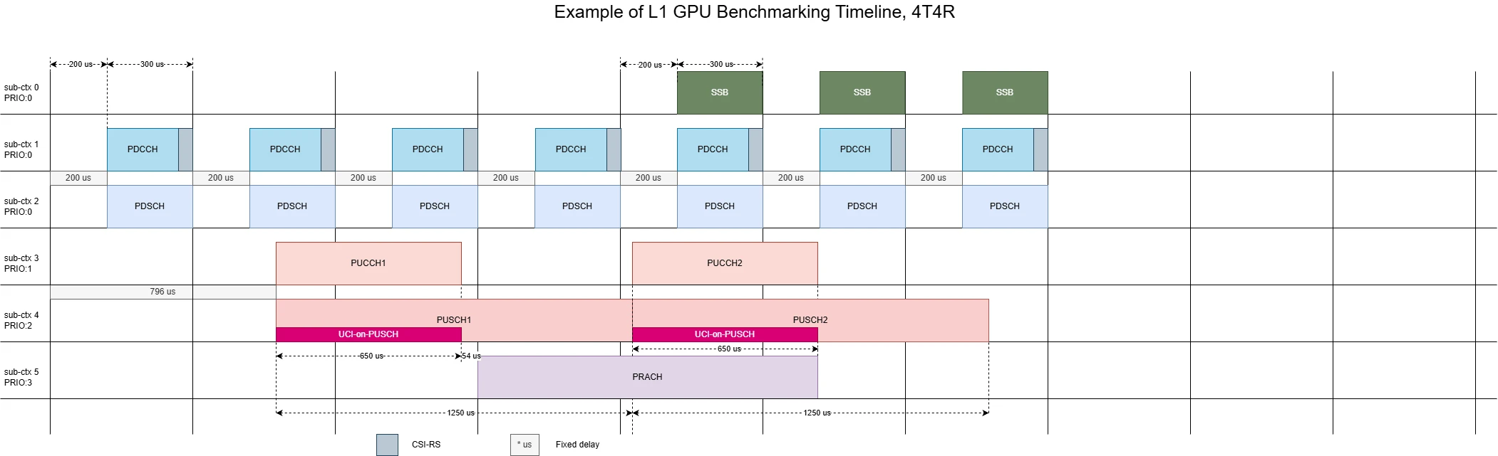
Figure B.1: L1 GPU benchmarking timeline example (PUSCH O-RAN 7.2a split, 4T4R, TDD pattern DDDSUUDDDD)

Appendix C: SM Tuning Example#

SM tuning is an important step during the benchmarking process for performance maximization.
The inputs to the SM tuning step are the total number of available SMs on the used GPU, e.g., 82 SMs on the GB203 GPU which is based on the second-generation Blackwell architecture, and the YAML configuration file which contains the benchmarking details such as workload, timeline, GPU frequency and power. The output of the SM tuning step should be an optimized SM allocation that maximizes benchmarking performance.
An optimized SM allocation is defined as follows: When a cell count of N generates a ref_check PASS, see Section 14.3 on test workflow, and the latency measurements are as close as possible to the latency budget for each channel, and when a cell count of N+1 generates a ref_check FAIL for multiple channels.
In the remaining of this section, we provide sample measurement results to demonstrate the SM tuning results. The measurement results in this appendix should not be considered as RANPerf benchmarking KPIs of the particular platform.
Figure C.1 shows the latency CDF (cumulative distribution function) graphs of different channels against the latency constraint of each channel in the example of a benchmarking scenario with the following inputs:
- DL offset of 200 µs and latency budget of 300 µs
- UL PUSCH1/PUSCH2 latency budget of 1,200/1,219 µs
- UCI latency budget of 615 µs
In each latency graph, there are three curves plotted: The blue curve corresponding to a cell count of N=17 cells, the red curve corresponding to a cell count of N+1=18 cells, and the black line which represents the latency constraint applicable to the particular graph.
As shown in the leftmost graph of the first and third row of graphs in Figure C.1, both PUSCH1 and PDSCH channels fail for a cell count of N+1=18. Although all other channels pass for both N=17 and N+1=18, see the rest of the graphs in Figure C.1, the cell count that meets all latency requirements is N=17, i.e., a cell count of N=17 would generate a ref_check PASS for the benchmarking scenario of Figure C.1. As already mentioned above, note that this cell count should not be treated as the cell capacity RANPerf benchmarking KPI of the particular platform.
Regarding the actual SM allocation, we can see from the titles of the graphs in Figure C.1 that PUSCH1/PUSCH2 channels are allocated 66 SMs each, PUCCH is allocated 10 SMs, PRACH is allocated 8 SMs, while PDSCH is allocated 46 SMs and PDCCH+CSI-RS are allocated 8 SMs. Please note that in addition to the allocated SMs, the titles of the graphs in Figure C.1 provide information on the priority of each channel according to the TDD priorities listed in Table B.3 of Appendix B. Also note that, in general, SM allocation would have different meaning depending on whether MPS or Green Contexts is used.
The following tips can be regarded as general guidance on SM allocation for enabling an efficient SM tuning process:
- Allocate a minimum of 8 SMs per channel.
- Initiate your SM tuning process by setting the number of SMs for PUSCH and PDSCH, which are the most processing-intensive channels, to approximately equal to 80% and 60%, respectively, of the total number of available SMs; in the benchmarking scenario of Figure C.1, the total number of available SMs is 82, while the number of SMs allocated to PUSCH and PDSCH is 66 and 46, respectively, which correlates well with the general guidance.
- To accelerate the SM tuning process, the latency tests can be run for a smaller number of slots and the number of SMs can be updated before the next set of latency tests are run after drawing the CDFs and determining how the latency CDF of each channel compares to its constraint.
- The latency tests should be eventually run for the higher number of slots to verify that all channels pass the reference check when the tentative optimized SM allocation is determined.

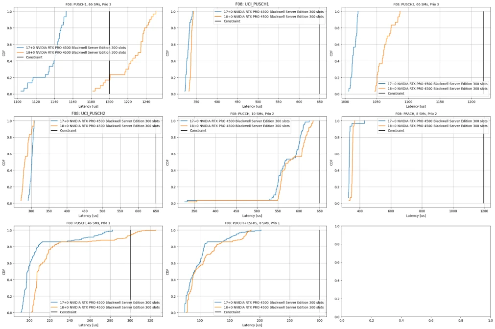
Figure C.1: Measurement results demonstrating the process of SM tuning

Appendix D: DL and UL Channel Configuration#

In Appendix D, we describe the frame structure and the key features of each supported channel for a typical multichannel test example using TDD pattern DDDSUUDDDD, 30 kHz SCS (subcarrier spacing)/0.5 ms slot duration, 100 MHz channel bandwidth (273 PRBs), 4T4R, 24 cells, and channels PDCCH, PDSCH, CSI-RS, PUSCH, PUCCH, PRACH, and UCI-on-PUSCH.

Figure D.1 shows the 40-slot alternating frame sequence for the used TDD pattern. In the following, the first 20 slots (slot 0 to slot 19) of each 40-slot sequence will be referred to as Group A, while the last 20 slots (slot 20 to slot 39) of each 40-slot sequence will be referred to as Group B. Note that slot numbering is 0-based.

Symbols 3 and 13 in each group are special symbols (S-slots) with the first 6 OFDM symbols dedicated for DL transmission, the next 4 symbols used as guard for DL/UL switching, and the last 4 symbols used for UL transmission (typically dedicated to SRS transmission).

Symbols 4 and 14 in each group are used for UL transmission (U-slots) and do not contain PRACH transmission; symbols 5 and 15 are also U-slots but contain PRACH transmission.

Figure D.1: 40-slot alternating frame sequence for the typical multichannel test pattern described in Appendix D; the slot number is calculated as mod(i,20), where i is the SFN (system frame number) that runs from 0 to 39 (from 0 to 19 for Group A and from 20 to 39 for Group B)

Although both Group A and Group B carry PDSCH, PDCCH, and CSI-RS channels, the CSI-RS channel in Group A carries both TRS and CQI CSI-RS (CSI-RS signal that is used for calculating CQI) while only TRS is transmitted in Group B. Figures D.2 and D.3 show how the D-slot is configured for Group A and Group B, respectively. Note that TRS is shown to be transmitted in symbols 5, 6, 9, and 10 in Figures D.2 and D.3, which corresponds to the transmission pattern in odd cells; in even cells, TRS would be transmitted in slots 6, 7, 10, and 11 (1-slot offset compared to TRS transmission in odd cells).

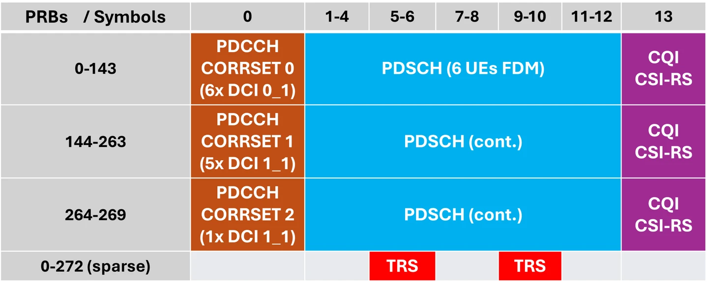
Figure D.2: D-slot channel configuration for Group A (first 20 slots of the alternating 40-slot frame sequence)

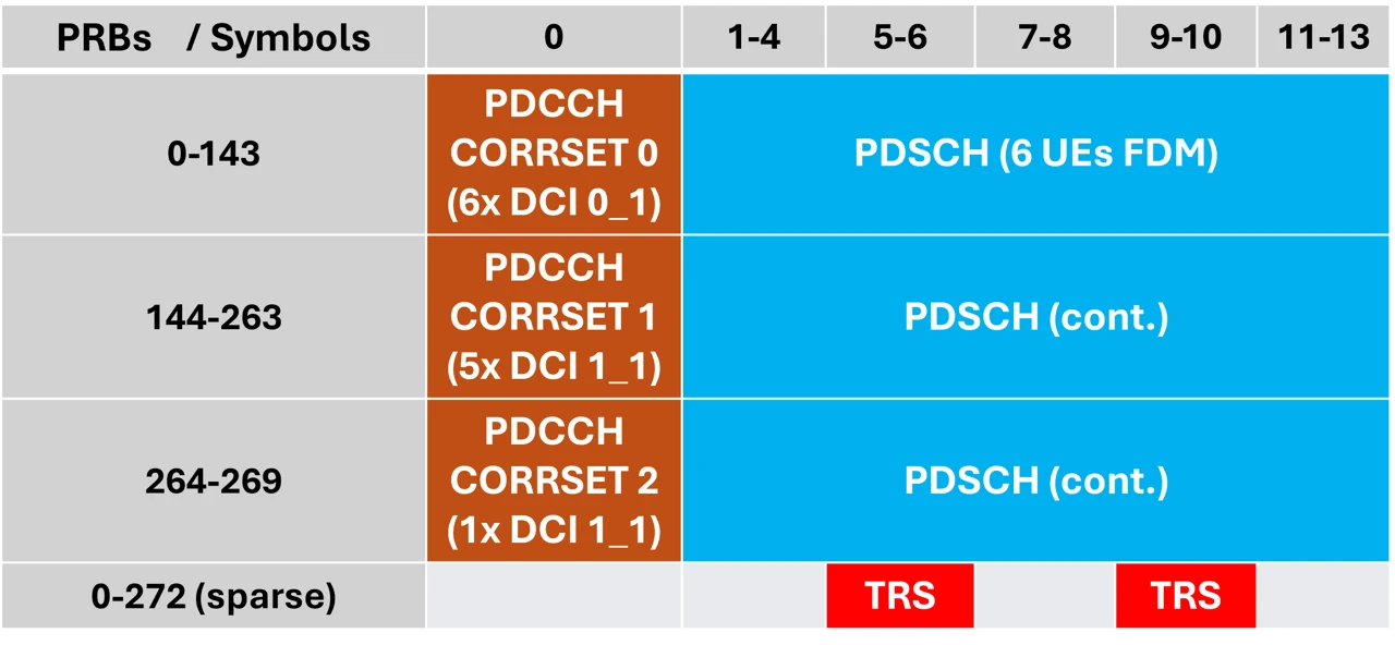
Figure D.3: D-slot channel configuration for Group B (last 20 slots of the alternating 40-slot frame sequence)

Figure D.4 shows the S-slot channel configuration where only a short, 5-symbol PUSCH channel is transmitted; the remaining 8 symbols (symbols 6-13) are dedicated for GP (guard period) and UL transmission (typically dedicated to SRS transmission).

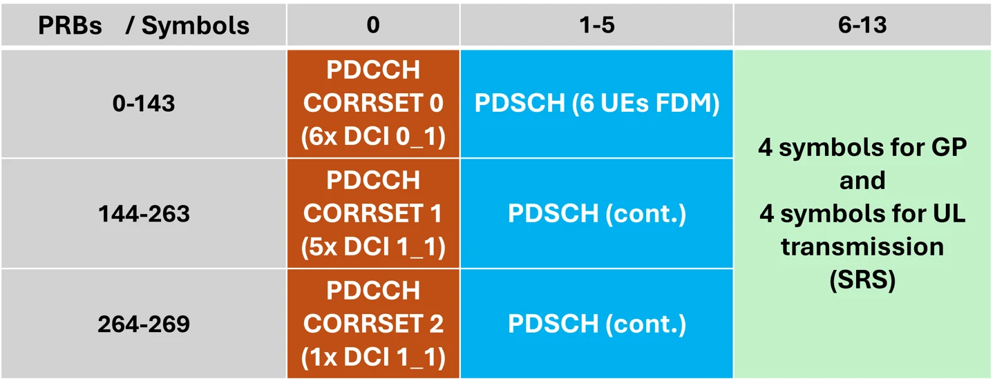
Figure D.4: S-slot channel configuration

As shown in Figure D.1, slots 4, 5, 14, and 15 in both Group A and Group B are U-slots. Slots 4 and 14 do not contain PRACH transmission, while slots 5 and 15 do. This difference is shown in Figure D.5 (valid for slots 4 and 14) and Figure D.6 (valid for slots 5 and 15), while the details of the common channels transmitted in the U-slots, i.e., PUCCH and PUSCH, are also described. Note that the PUCCH configuration is identical for all U-slots, while the size of PUSCH in slots 5 and 15 is smaller due to the transmission of PRACH which is accommodated in the last 12 PRBs (PRBs 261 to 272) of the slot; as 8 UEs are transmitted in each PUSCH allocation, each UE occupies 30, 31, or 32 PRBs (for a total of 252 PRBs) in Figure D.5 and 29, 30, or 31 (for a total of 240 PRBs) in Figure D.6. Finally, note that PRACH is transmitted only along the first 12 OFDM symbols (symbols 0 to 11) of U-slots 5 and 15.

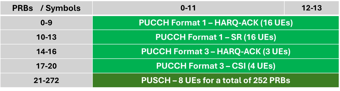
Figure D.5: U-slot channel configuration of slots 4 and 14 of each group in the 40-slot alternating 40-slot frame sequence, see Figure D.1

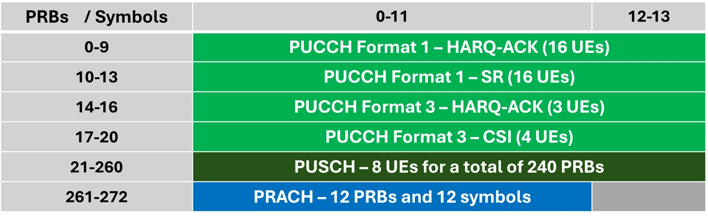
Figure D.6: U-slot channel configuration of slots 5 and 15 of each group in the 40-slot alternating 40-slot frame sequence, see Figure D.1

In the remaining part of Appendix D, we list the main parameters of all DL and UL supported channels in the considered multichannel test example in addition to the parameters shown in Figures D.1 to D.6. As the list of parameters is not exhaustive, the user is referred to the YAML configuration file of each test for the complete list of parameters used to configure each DL and UL channel.

PDSCH:
- MCS index: 27 (0-based), which corresponds to spectral efficiency of 7.4063 (256-QAM modulation and 948/1024 code rate), see Table 5.1.3.1-2 of 3GPP TS 38.214 (5G; NR; Physical layer procedures for data, Release 16)
- Number of UEs: 6, where each UE is allocated 46 or 43 PRBs for a total of 273 PRBs for the used 100 MHz bandwidth, see Figure D.1 and Figure D.2 for slots in Group A (over 12 symbols in the time domain) and slots in Group B (over 13 symbols in the time domain), respectively
- Number of layers per UE: 4
- DMRS configuration: Type 1 with one additional symbol, which means that two DMRS symbols are transmitted per slot, while 2 CDM groups are supported
- Precoding: Identity precoder enabled (enableIdentityPrecoderMap = 1)
- Note: As TRS is transmitted every 4th PRB, 204 PRBs in each TRS symbol of each slot are used for PDSCH transmission
PDCCH:
- CORESET 0: DCI Format 0_1 (UL grants), 1 OFDM symbol duration, 6 DCIs, Aggregation Level 4, 24 CCEs, Interleaved CCE mapping, REG bundle size of 2, Interleaver size of 2
- CORESET 1: DCI Format 1_1 (DL assignments), 1 OFDM symbol duration, 5 DCIs, Aggregation Level 4, 20 CCEs, Interleaved CCE mapping, REG bundle size of 2, Interleaver size of 2
- CORESET 2: DCI Format 1_1 (DL assignments), 1 OFDM symbol duration, 1 DCI, Aggregation Level 1, 6 PRBs, Non-interleaved CCE mapping, REG bundle size of 2
- Payload size: 39 bits per DCI, 12 DCIs per slot
CSI-RS:
- TRS:
  - In even cells: Always transmitted in symbols 6, 7, 10, and 11 of each slot, sparse transmission (every 4th PRB), beam index 0 for slots in Group A, see Figure D.2, and beam index 5 for slots in Group B, see Figure D.3
  - In odd cells: Always transmitted in symbols 5, 6, 9, and 10 of each slot, sparse transmission (every 4th PRB), beam index 0 for slots in Group A, see Figure D.2, and beam index 5 for slots in Group B, see Figure D.3
- CQI CSI-RS: Transmitted in symbol 13 of each slot in Group A, see Figure D.2, Density=3 (3 REs are allocated to CSI-RS per PRB), beam indices 1-4
PUSCH:
- MCS index: 27 (0-based), which corresponds to spectral efficiency of 7.4063 (256-QAM modulation and 948/1024 code rate), see Table 5.1.3.1-2 of 3GPP TS 38.214 (5G; NR; Physical layer procedures for data, Release 16)
- Number of UEs: 8, where each UE is allocated 30, 31, or 32 PRBs in slots 4 and 14 (where no PRACH is transmitted, see Figure D.5) and 29, 30, or 31 PRBs in slots 5 and 15 (where PRACH is transmitted, see Figure D.6)
- Number of layers per UE: 2
- DMRS configuration: Type 1 with one additional symbol, which means that two DMRS symbols are transmitted per slot, while 2 CDM groups are supported
- LDPC decoder: Uses a fixed number of 10 iterations
- UCI (UCI-on-PUSCH): Can be enabled using a specific profile
PUCCH (see Figures D.5 and D.6):
- Format 1, HARQ-ACK: 16 UEs, 2 UEs/PRB on PRBs 0–5 via CS/OCC; 1 UE/PRB on PRBs 6–9
- Format 1, SR: 16 UEs, 4 UEs/PRB via CS/OCC, SR flag set
- Format 3, HARQ-ACK: 3 UEs, 1 UE/PRB, 1-bit HARQ payload
- Format 3, CSI report: 4 UEs, 1 UE/PRB, 64-bit CSI payload
PRACH:
- Configuration 158, see Table 6.3.3.2-3 of 38.211 (5G; NR; Physical channels and modulation, Release 18), ZCZ (zero correlation zone) 0, SCS 30 kHz, Beam indices 0 and 1

Appendix E: DL and UL Spectral Efficiency Calculation#

Introduction#

In Appendix E, we calculate the DL and UL spectral efficiency for the TDD test example described in Appendix D. Although different channel configurations would lead to slightly different spectral efficiency values, the calculations in this appendix are representative for a single-user (SU)-MIMO TDD system that operates close to a mode generating the highest possible DL and UL throughput for the assumed TDD pattern.

To calculate the TDD DL or UL spectral efficiency, we need to:

Calculate the total number of useful data bits transmitted in the DL or UL by considering the DL or UL control overhead.
Calculate the effective channel bandwidth by considering the TDD DL:UL ratio of the assumed TDD pattern.
The DL or UL spectral efficiency is defined by the ratio of the DL or UL useful data bits divided by the reference TDD pattern time duration and the DL or UL effective channel bandwidth.
Note: To facilitate the spectral efficiency calculations, we consider the reference TDD pattern of Figure D.1 (7 D-slots, 1 S-slot, and 2 U-slots, 5 ms time duration).

DL Spectral Efficiency Calculation#

Number of PRBs used for data transmission:
- D-slot, Group A: 8 full symbols (273 PRBs each) and 4 partial symbols due to TRS transmission (204 PRBs each), leading to a total of 3,000 PRBs.
- D-slot, Group B: 9 full symbols (273 PRBs each) and 4 partial symbols due to TRS transmission (204 PRBs each), leading to a total of 3,273 PRBs.
- D-slot, average over Group A and Group B: 3,136.5 PRBs.
- S-slot: 4 full symbols (273 each) leading to a total of 1,092 PRBs.
- Total number of PRBs: 7*3,136.5 + 1*1,092 = 23,047.5.
Number of REs used for data transmission (12 REs/PRB):
- 23,047.5 * 12 = 276,570.
For MCS index 27 (256-QAM modulation, 948/1024 code rate) and 4 layers per UE, the total number of useful data bits is: 276,570 * 8 * (948/1024) * 4 ~= 8.2*10⁶ bits.
Effective channel bandwidth (7 D-slots and 1 S-slot with 6 DL symbols): 100 MHz * (7*14+1*6) / (10*14) = 74.3*10⁶ Hz.
DL spectral efficiency = 8.2*10⁶ / (5*1E-03 * 74.3*10⁶) ~= 22.1 b/s/Hz

UL Spectral Efficiency Calculation#

Number of PRBs used for data transmission:
- U-slot, Slots 4 or 14: 252 PRBs over 12 symbols, leading to a total of 3,024 PRBs.
- U-slot, Slots 5 or 15: 240 PRBs over 12 symbols, leading to a total of 2,880 PRBs.
- U-slot, average over all slot types: 2,952 PRBs.
- S-slot: No PRBs for data transmission (all symbols allocated for SRS transmission).
- Total number of PRBs: 2 * 2,952 = 5,904.
Number of REs used for data transmission (12 REs/PRB):
- 5,904 * 12 = 70,848.
For MCS index 27 (256-QAM modulation, 948/1024 code rate) and 2 layers per UE, the total number of useful data bits is: 70,848 * 8 * (948/1024) * 2 ~= 1.1*10⁶ bits.
Effective channel bandwidth (2 U-slots and 1 S-slot with 4 UL symbols): 100 MHz * (2*14+1*4) / (10*14) = 22.9*10⁶ Hz.
UL spectral efficiency = 1.1*10⁶ / (5*1E-03 * 22.9*10⁶) ~= 9.2 b/s/Hz