Gas Tank Filling - Transient Conjugate Heat Transfer#
The simulation workload for “tank filling” falls into two distinct categories depending on the fluid: liquid filling (e.g., automotive fuel, water) or high-pressure gas filling (e.g., hydrogen/CNG). While both are “filling,” the computational physics and workload challenges are completely different.
Gas/Hydrogen Tank Filling (The “Thermal” Workload)#
This is critical for the green energy industry (Hydrogen FCEVs). The challenge here is thermodynamics, not splashing. Compressing gas into a tank generates massive amounts of heat (heat of compression + Joule-Thomson effect).
The core physics:
Compressible flow: Density changes drastically as pressure rises.
Real gas models: Solvers must use complex equations of state to model how hydrogen behaves at high pressure.
Conjugate heat transfer: The simulation must calculate how heat moves from the hot gas into the plastic liner through the carbon fiber wrapping to the outside air.
Computational challenges:
Long time scales: Unlike a 3-second liquid splash, a hydrogen fill takes 3-5 minutes. Simulating this fully in 3D is very expensive.
Fluid-solid coupling: The solver must solve fluid equations (inside) and solid thermal equations (tank wall) simultaneously.
What engineers look for:
Overheating: The tank temperature must stay within safety limits for the tank materials. The simulation predicts if the fill rate is too fast, causing the gas to get too hot.
Liquid Tank Filling (The “Free Surface” Workload)#
The primary challenge here is geometry and interface tracking. You are simulating a heavy fluid crashing into a light fluid, creating complex splashing, bubbling, and turbulence.
The core physics:
Multiphase flow (VOF): Solvers use the Volume of Fluid (VOF) method to track the sharp interface between air and liquid. It solves a transport equation for the “volume fraction” in every cell.
Turbulence: Models like k-epsilon or LES (Large Eddy Simulation) are used to predict how the incoming jet breaks up.
Computational challenges:
Transient (time-dependent): The simulation must run in tiny time increments to capture the fluid motion accurately.
Adaptive meshing: To see droplets and bubbles, the mesh must be incredibly fine at the liquid surface. Advanced solvers use Adaptive Mesh Refinement (AMR) to dynamically increase resolution.
Courant number constraints: The simulation time-step is limited by the speed of the fluid. If the liquid moves too fast across a mesh cell, the simulation crashes, forcing the solver to take even smaller (more expensive) time steps.
What engineers look for:
Blowback/splash-back: Does the fuel splash up the pipe and trigger the nozzle to shut off early?
Air entrapment: Does air get trapped in “pockets” inside the tank, preventing it from filling to 100% capacity?
This example trains and runs a DoMINO model on transient conjugate heat transfer simulations. Raw CFD solver dumps (VTU per timestep) are preprocessed into NPZs, then the model predicts surface and volume fields for multiple future timesteps in one shot. Inference can write VTKs for inspection.
Problem Description#
This use case models compressed natural gas (CNG) tank filling with optional active cooling. The filling process is transient, compressible, and involves conjugate heat transfer between the gas, tank wall, and cooling coil (if present). During filling, gas compression raises temperature, which limits how much mass can be stored and can raise thermal stress concerns. The model aims to capture the evolving thermal and flow fields over the full fill horizon.
The dataset was generated by varying:
Tank final pressure (200, 250, or 300 bar).
Fill duration (60, 90, or 120 seconds).
Inlet gas temperature (-40, -10, or 25 C).
Cooling coil configuration (none, front, mid, back).
Inputs, outputs, and conditioning#
The model is conditioned on both geometry and global operating parameters. The selection mirrors the quantities that materially affect compression heating and heat transfer during a fill.
Inputs:
Surface mesh from the initial timestep (
sim_0), which encodes the tank geometry, internal components, and coil layout.Global parameters that define the fill scenario (pressure target, inlet temperature, duration, and coil position).
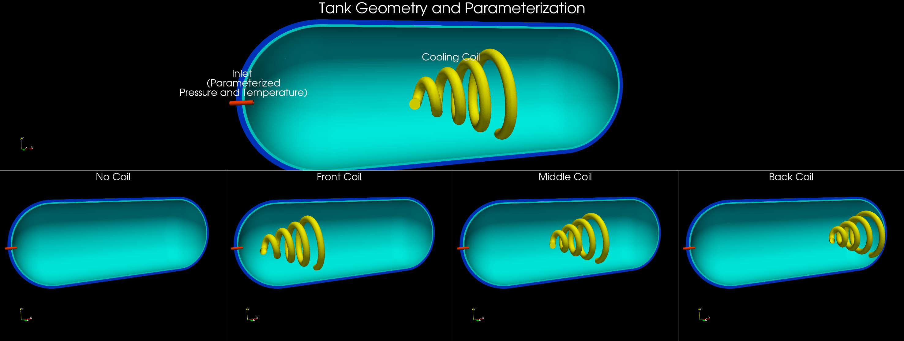
Tank filling simulation snapshot#
Global parameters in this example:
pressure_bar: Final tank pressure target (e.g., 200/250/300 bar).inlet_temperature_C: Inlet gas temperature (e.g., -40, -10, 25 C).run_time_s: Fill duration (e.g., 60/90/120 s).coil_position: Categorical coil placement (0 none, 1 front, 2 mid, 3 back).
These are parsed from the simulation folder name in process_data.py and provided alongside geometry to the model. If you use different parameters or a different naming convention, update both parse_params and variables.global_parameters in the config.
Outputs:
Surface fields: pressure, temperature, wall shear stress magnitude, and heat flux.
Volume fields: pressure, temperature, velocity, and heat flux.
These outputs are chosen to capture the primary thermal and flow responses of the tank during filling, and to enable downstream calculations such as temperature statistics, heat fluxes on internal surfaces, and flow structure visualization. The transient horizon is predicted in one shot, meaning all future timesteps (for example, 12-24) are produced in a single forward pass, similar to a steady-state prediction rather than an autoregressive rollout.
Data layout#
Users can structure the data generated from their numerical solvers in the following schema to use this recipe on their own data. The dataset used for this example is not yet available for public training but will be released soon.
Raw simulations (per case) are laid out as:
<raw_dir>/<sim_name>/<sim_name>/
├─ sim_0/                   # initial timestep (geometry only)
│  ├─ sim_0.boundaries.vtu  # surface mesh (boundary triangles)
│  └─ FLUID0_REG0.vtu, SOLID*.vtu  # volume regions (cell-centered)
├─ sim_1/, sim_2/, ..., sim_N/   # subsequent timesteps with surface/volume fields
└─ probe_points_*.csv, inlet_*.csv, residuals.csv ... (aux files, ignored)
process_data.py traverses both levels of folders to find sim_* timesteps, packs each simulation into a single NPZ, and writes scaling stats to <processed_dir>/stats.
Simulation naming and global parameters#
The default preprocessing extracts global parameters from the simulation folder name. It expects a pattern like:
<prefix>_<pressure>bar_<temperature>C_<runtime>s
The <prefix> can include a coil tag (for example, frontcoil), which is mapped to variables.global_parameters.coil_position in conf/config.yaml. If your dataset uses different naming or parameters, update parse_params in process_data.py and the variables.global_parameters section in the config.
Key scripts#
process_data.py— preprocess raw VTU folders into NPZs (<processed_dir>/train|val) and stats. Skips sims already processed.train.py— trains DoMINO using the processed NPZs and writes checkpoints/tensorboard to${project.output_root}.inference.py— runs a trained checkpoint on raw VTU folders, writing per-timestep surface.vtpand volume.vtufiles withpred_*(and optionalgt_*) fields.
Quickstart#
Configure paths in
conf/config.yaml, or pass overrides in the commands below.Preprocess:
python process_data.py data.raw_dir=/path/to/raw_simulations \
  data.processed_dir=/path/to/processed_npz
Train:
python train.py data.processed_dir=/path/to/processed_npz \
  project.output_root=/path/to/outputs
Checkpoints land in
${project.output_root}/checkpoints; tensorboard in${project.output_root}/tensorboard.Inference to VTK:
python inference.py data.raw_dir=/path/to/raw_simulations \
  data.processed_dir=/path/to/processed_npz \
  inference.checkpoint=/path/to/outputs/checkpoints \
  inference.output_dir=/path/to/outputs/inference
Writes per-timestep
surface/*.vtpandvolume/<region>.vtufiles under${inference.output_dir}/<sim_name>/.
Training approach (one-shot forecasting)#
Each sample uses geometry from
sim_0and concatenates fields fromsim_1..sim_Tinto a single target tensor.The target is stacked by timestep in the channel dimension, so the model predicts the entire horizon in one forward pass (no autoregressive rollout).
The number of predicted steps is controlled by
data.future_steps; smaller simulations are padded and masked so training still works.Use
model.model_type: surface | volume | combinedto control which outputs are trained.
Notes and tips#
data.val_fractionordata.splits.train/valcontrols the train/val split.Multi-GPU Support: Compatible with
torchrunor MPI for distributed training.Inference runs on a single GPU per process; launch multiple processes or split simulations to parallelize.
train.resume: true/falsecontrols checkpoint loading; default is resume.train.amp: trueenables autocast + GradScaler on CUDA.Normalization expects stats in
<processed_dir>/stats; missing stats will raise unless you disablemodel.normalization.Inference uses the same stats by default; override with
inference.stats_dirif needed.