Bilateral Filter#

Overview#

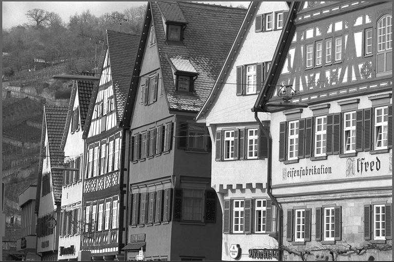
The Bilateral Filter is a non-linear, edge-preserving smoothing filter that combines spatial and range filtering to achieve intelligent noise reduction. It is commonly used in computer vision pipelines for tasks such as image denoising, detail enhancement, and as a preprocessing step for edge detection and feature extraction.

Input Image	Output Image

Bilateral Filter Parameters: sigmaRange = 50, sigmaSpace = 1.7, kernel size = 5x5

Reference Implementation#

The reference implementation of this bilateral filter algorithm is based on VPI.

The bilateral filter is defined as:

\[I'(p) = \frac{1}{W_p} \sum_{q \in \Omega} I(p)k_r(\|I(q)-I(p)\|)k_s(\|p-q\|)\]

and the normalization term, W, is defined as:

\[W_p = \sum_{q \in \Omega} k_r(\|I(q)-I(p)\|)k_s(\|p-q\|)\]

where:

\(I\) and \(I'\) are the input and output images, respectively.
\(k_r\) and \(k_s\) are the range and space kernels, respectively, defined as the following non-normalized Gaussian functions:

\[ \begin{align}\begin{aligned}k_r(p) = e^{-\frac{\|p\|^2}{2\sigma_r^2}}\\k_s(p) = e^{-\frac{\|p\|^2}{2\sigma_s^2}}\end{aligned}\end{align} \]

\(\sigma_r\) controls the intensity range that is smoothed out. Higher values will lead to textures and details being smoothed out. The \(\sigma_r\) value should be selected with the dynamic range of the image pixel values in mind.
\(\sigma_s\) controls spatial smoothing factor. Higher values will lead to more smoothing.

More information can be found in [1].

Implementation Details#

Limitations#

The current implementation has the following limitations:

Only supports 3x3, 5x5, and 7x7 kernel sizes.
Only supports uint8 input and output data types.
Only supports NVCV_BORDER_CONSTANT and NVCV_BORDER_REPLICATE border modes.

Dataflow Configuration#

2 RasterDataFlow(RDF) are needed:

1 input RDF is used to split the input tensor into tiles and transfer them with overlapped regions for the filtering from DRAM into circular buffer in VMEM.
1 output RDF is used to transfer the output tensor by tiles from ping pong buffer in VMEM to DRAM.

Buffer Allocation#

6 VMEM buffers are needed:

Input buffers:

1 input image buffer with circular buffering for each tile of the input image.
1 weight table buffer for pre-computed bilateral filter weights.
1 weight table replicate buffer for efficient weight lookup.

Intermediate buffers:

1 value sum buffer for accumulated weighted values.
1 weight sum buffer for accumulated kernel weights.

Output buffers:

1 output image buffer with double buffering for each tile of the output.

Kernel Implementation#

- 3x3 kernel (radius=1, radius^2=1)
 ┌──────┐
 │/ 1 / │
 │1 0 1 │ → space2Param[2] = {1, 0}
 │/ 1 / │
 └──────┘

- 5x5 kernel (radius=2, radius^2=4)
 ┌──────────┐
 │/ / 4 / / │
 │/ 2 1 2 / │
 │4 1 0 1 4 │ → space2Param[4] = {4, 2, 1, 0}
 │/ 2 1 2 / │
 │/ / 4 / / │
 └──────────┘

- 7x7 kernel (radius=3, radius^2=9)
 ┌──────────────┐
 │/ / / 9 / / / │
 │/ 8 5 4 5 8 / │
 │/ 5 2 1 2 5 / │
 │9 4 1 0 1 4 9 │ → space2Param[7] = {9, 8, 5, 4, 2, 1, 0}
 │/ 5 2 1 2 5 / │
 │/ 8 5 4 5 8 / │
 │/ / / 9 / / / │
 └──────────────┘

Therefore, we can pre-compute all possible cases of the bilateral filter kernel and create a lookup table. During computation, we use \(\|I(q)-I(p)\|\) and \(\|p-q\|\) as indices to look up the corresponding kernel weights from the lookup table to generate the bilateral filter kernel.

Additionally, to optimize performance on VPU hardware, our implementation uses a fixed-point quantization method for the filter weights. The floating-point weights are converted to uint8 type using 7 fractional bits (Q1.7 format). The quantization process is implemented as follows:

\[\text{weight}_{\text{fixed}} = \text{clamp}(\text{round}(\text{weight}_{\text{float}} \cdot 2^7), 0, 255)\]

This quantization allows for efficient computation while maintaining sufficient precision for the bilateral filter operation.

The bilateral filter implementation is divided into two stages:

Accumulation Stage:

For each pixel in the tile:
- Compute \(\|I(q)-I(p)\|\) and \(\|p-q\|\).
- Retrieve kernel weights from the lookup table.
- Accumulate the sum of weighted values and the sum of kernel weights.
We use two agens to handle the irregular data access pattern (see Figure 1). The green area represents the valid kernel region (where Euclidean distance is less than or equal to the kernel radius), while the white area represents the invalid region. For the valid region, we use the corner agen to load four relatively independent kernel weights, and the central agen to load the kernel weights in the central region.

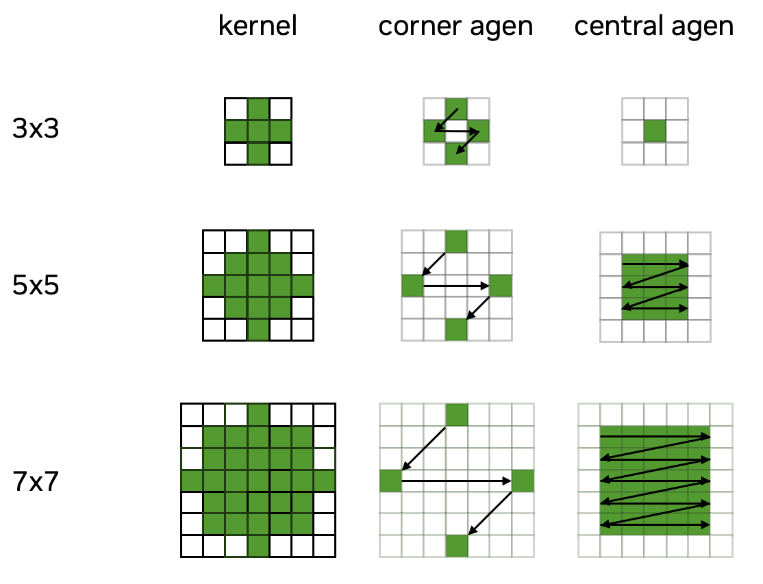
../../_images/bilateral-filter-agen-pattern.png — Figure 1: Agen access pattern for bilateral filter kernel.#

Division Stage:
- Convert both the sum of weighted values and the sum of kernel weights to float type.
- Perform division on the sum of weighted values and the sum of kernel weights to obtain the final results.
- Convert the results back to uint8 type while storing it.

Performance#

Execution Time is the average time required to execute the operator on a single VPU core. Note that each PVA contains two VPU cores, which can operate in parallel to process two streams simultaneously, or reduce execution time by approximately half by splitting the workload between the two cores.

Total Power represents the average total power consumed by the module when the operator is executed concurrently on both VPU cores.

For detailed information on interpreting the performance table below and understanding the benchmarking setup, see Performance Benchmark.

ImageSize	KernelSize	DataType	Execution Time	Submit Latency	Total Power
1920x1080	3x3	U8	0.967ms	0.031ms	12.324W
1920x1080	5x5	U8	1.310ms	0.038ms	12.405W
1920x1080	7x7	U8	3.385ms	0.048ms	11.619W

Reference#

NVIDIA VPI Documentation: https://docs.nvidia.com/vpi/algo_bilat_filter.html