WarpPerspective

Overview

The WarpPerspective operator applies perspective or affine transformation to an image, allowing for correction of perspective distortion or geometric transformation. The transformation is defined by a 3x3 matrix, which maps output pixel coordinates to input coordinates. This operator supports both nearest neighbor and bilinear interpolation methods. Typical use cases include correcting camera misalignment, simulating viewpoint changes, or performing projective transformations in computer vision pipelines. After applying this operator, sometimes cropping and scaling are followed to remove the regions interpolated from out-of-bounds pixels.

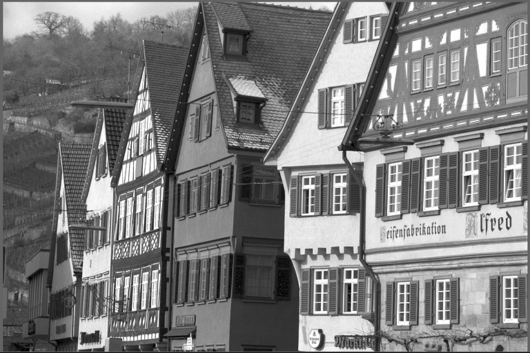
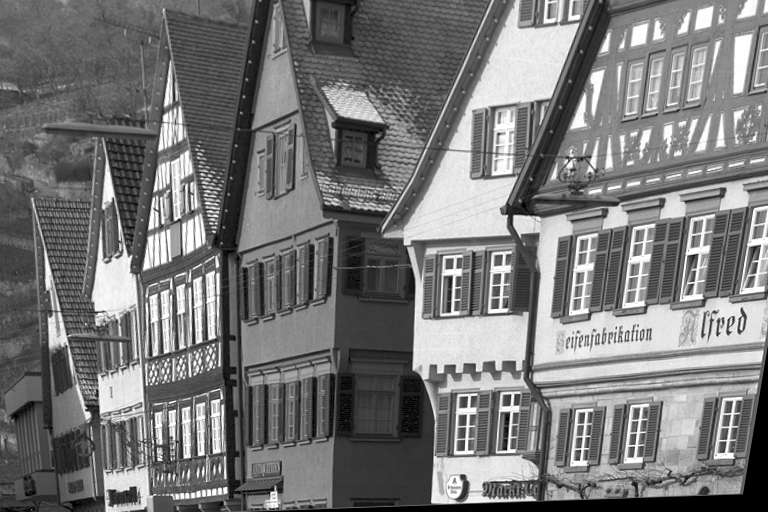
See the images below, the left one is input image, and the right one is the output of WarpPerspective operator. Black regions from right image are interpolated from out-of-bounds input pixels. In order to have better visualization effect, scale factor is 1.1 for both width and height, and tiny rotation is also added. For most real use cases, the scale factor may not be so large, and the rotation angle may even close to 0.

Figure 1: Sample input image (left) and its warped image (right)

Algorithm Description

The operator divides the output image into tiles of size 64x54 (TILE_W x TILE_H). The tile size can be adjusted based on customer’s requirement, 64x54 here is convenient for 1920x1080 sample resolutions. For each output tile, the corresponding input region is computed using the 3x3 inverse warp matrix. The transformation is applied as follows:

\[\begin{split}\begin{bmatrix} x' \\ y' \\ z' \end{bmatrix} = \text{invWarpMatrix} * \begin{bmatrix} x \\ y \\ 1 \end{bmatrix}\end{split}\]

For perspective transformation, the input coordinates \((x'/z', y'/z')\) are then used to sample the input image using the selected interpolation method. If this transformation is also affine, the third row of the invWarpMatrix is \((0, 0, 1)\). It’s easy to know \(z'\) is always 1 and \((x', y')\) can be directly utilized as input coordinates. Refer to [1] and [2] for more details.

Implementation Details

For a rectangle output region, the necessary input region is a quadrilateral. When transferring input regions through DMA, the actual bounding boxes encompassing the quadrilaterals are transferred. Here the term input tiles will only stand for input bounding boxes in the following paragraphs. See the illustration picture below for the input quadrilateral when performing perspective transformation like Figure 1. The quadrilateral boundary is highlighted in red, and only ones inside the original input image are presented.

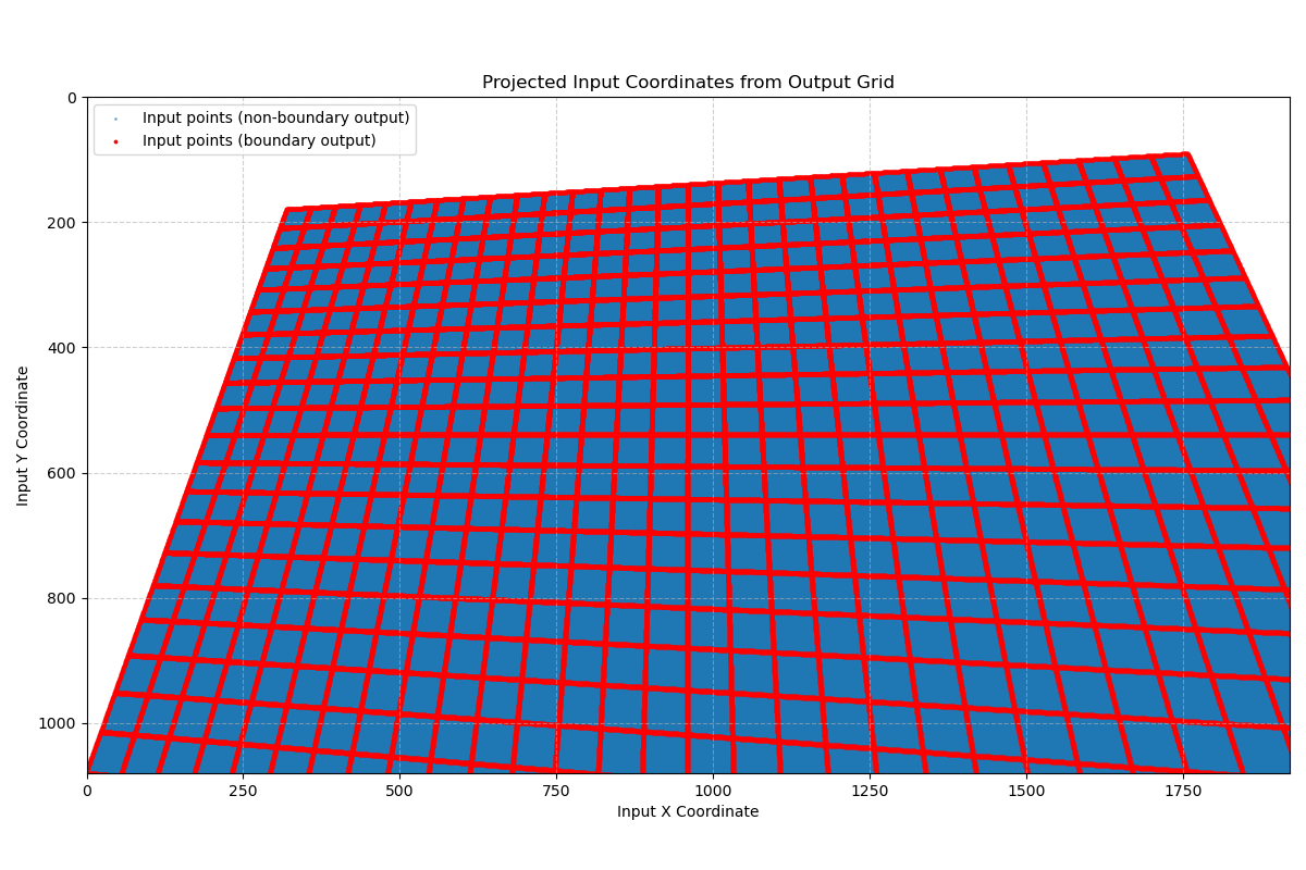
Figure 2: Input quadrilaterals

Limitations

• Output image width and height must be divisible by TILE_W(64) and TILE_H(54).

• Only U8 and NV12 formats are supported.

• Only constant border mode is supported for out-of-bounds pixels.

• The input and output image format must match.

• The input and output image sizes must be specified at operator creation and cannot change.

• Customers can update the inverse warping matrix at submission time for different cameras or frames.

Note at Orin, VPU has 3 superbanks with 128KB for each to enable maximum VMEM load/store throughput. This application is VPU compute bound for typical use case, so all 3 superbanks should be utilized for internal VPU kernels for better performance. And 64KB is allocated for input tiles, considering to enable double buffering, 32KB is the maximum size for a single input tile. 32KB should handle most use cases as it’s 9x larger than output tile size, and sanity checking is also enabled to ensure every input tile size is smaller than 32KB.

Dataflow Configuration

Input tiles are transferred through GatherScatterDataflow(GSDF) and output ones are through SequenceDataFlow(SQDF).

GSDF is used to transfer input tiles from DRAM to VMEM. From Figure 2 it’s easy to aware that input tiles have various width and height, so GSDF is suitable here.

SQDF is used to transfer output tiles from VMEM to DRAM. Though the output tile is always TILE_W x TILE_H, the related input tiles may be fully out of input boundary. Under those cases, most of the VPU computations can be skipped, also the DMA transfer between VMEM and DRAM can be omitted. That helps boost the full frame performance, and SQDF is more suitable than RasterDataflow(RDF) in this scenario.

Coordinates Generation

For single plane U8 image, when generating input homography coordinates from output ones, all x/y/z dimensions are derived from linear combinations of inverse matrix row vectors and output ones. That means the calculations meet distributive law, and extracting the common part of steps can help reduce total VPU coordinates computation time.

Let’s assume output coordinates are \((x_{out}, y_{out}, 1)^T\), and it can be decomposed into combinations between the first tile’s coordinates \((baseX, baseY, 1)^T\) and delta vector \((tile\_idx * TILE\_W, tile\_idy * TILE\_H, 0)^T\). Note here \(x_{out}\) and \(y_{out}\) are short for \(x_{out}(i, j)\) and \(y_{out}(i, j)\) respectively, and \(i\) and \(j\) help locate a certain pixel from a tile. \(baseX\) and \(baseY\) are also short for \(baseX(i, j)\) and \(baseY(i, j)\). The \(tile\_idx\) and \(tile\_idy\) stand for tile sequence number at horizontal and vertical dimensions from a full frame viewpoint. The following equation tries to reflect the coordinates relationship between arbitrary output tiles and the first one.

\[\begin{split}\begin{bmatrix} x_{out} \\ y_{out} \\ 1 \end{bmatrix} = \begin{bmatrix} baseX + tile\_idx * TILE\_W \\ baseY + tile\_idy * TILE\_H \\ 1 + 0 \end{bmatrix}\end{split}\]

The input homography coordinates before normalization \((x', y', z')^T\) would be:

\[\begin{split}\begin{bmatrix} x' \\ y' \\ z' \end{bmatrix} = inverseWarpMatrix * (\begin{bmatrix} baseX \\ baseY \\ 1 \end{bmatrix} + \begin{bmatrix} tile\_idx * TILE\_W \\ tile\_idy * TILE\_H \\ 0 \end{bmatrix})\end{split}\]

Let’s define:

\[\begin{split}\text{BaseCords} = inverseWarpMatrix * \begin{bmatrix} baseX \\ baseY \\ 1 \end{bmatrix}\end{split}\]

\[\begin{split}\text{DeltaCords} = inverseWarpMatrix * \begin{bmatrix} TILE\_W \\ TILE\_H \\ 0 \end{bmatrix}\end{split}\]

\(BaseCords\) and \(DeltaCords\) are constant and can be calculated before tile processing. When having \(tile\_idx\) and \(tile\_idy\) for each tile, \((x', y', z')^T\) can be derived from \(BaseCords\) and \(DeltaCords\) quickly. Then do normalization through \((x_{in}, y_{in}, 1)^T = (x', y', z')^T / z'\).

When the transformation is affine, \(z'\) is always 1, so \((x', y', z')^T\) is same with \((x_{in}, y_{in}, 1)^T\). VPU will detect transformation type and simplify affine coordinates calculation.

For NV12 format, coordinates generation for luma plane is the same with single plane U8 image. For two interleaved chroma planes with 2x downscale for width and height, coordinates are generated via luma ones through \(((x1 + x2 + x3 + x4) * 0.25f - 0.5f) * 0.5f\). Here \(x1, x2, x3, x4\) are the 4 adjacent luma plane coordinates from top-left, top-right, bottom-left and bottom-right respectively.

Remapping

After finishing coordinates generation, the next step is remapping. CupvaSampler in PVA SDK is high-level abstraction for PVA’s Decoupled Lookup Table Unit (DLUT), which can handle lookup with fractional indices. Both nearest neighbor and bilinear interpolation are supported. Furthermore, the DLUT based remapping is independent of VPU once the sampler structure is configured, it can execute in parallel with coordinates generation of the next tile.

Performance

Different warping transformations would lead to huge performance variations. The performance below only reflects the transformations showed in the Overview section.

Execution Time is the average time required to execute the operator on a single VPU core. Note that each PVA contains two VPU cores, which can operate in parallel to process two streams simultaneously, or reduce execution time by approximately half by splitting the workload between the two cores.

Total Power represents the average total power consumed by the module when the operator is executed concurrently on both VPU cores.

For detailed information on interpreting the performance table below and understanding the benchmarking setup, see Performance Benchmark.

Transform	Interp	InputSize	OutputSize	ImageFormat	Execution Time	Submit Latency	Total Power
Affine	NN	1920x1080	1920x1080	U8	1.683ms	0.088ms	11.738W
Affine	NN	1920x1080	1920x1080	NV12_ER	2.734ms	0.135ms	11.638W
Affine	LINEAR	1920x1080	1920x1080	U8	1.667ms	0.093ms	11.738W
Affine	LINEAR	1920x1080	1920x1080	NV12_ER	2.732ms	0.135ms	11.638W
Perspective	NN	1920x1080	1920x1080	U8	2.000ms	0.090ms	11.638W
Perspective	NN	1920x1080	1920x1080	NV12_ER	3.042ms	0.134ms	11.254W
Perspective	LINEAR	1920x1080	1920x1080	U8	2.021ms	0.085ms	11.638W
Perspective	LINEAR	1920x1080	1920x1080	NV12_ER	3.044ms	0.134ms	11.638W

Reference

1. NVIDIA VPI Documentation: https://docs.nvidia.com/vpi/algo_persp_warp.html

2. OpenCV Documentation: https://docs.opencv.org/4.x/da/d54/group__imgproc__transform.html