HistogramEqualization#

Overview#

Histogram Equalization is an image processing technique used to enhance the contrast of images by effectively spreading out the most frequent intensity values in an image, i.e., stretching out the intensity range of the image. The method is particularly effective when the usable data of the image is represented by close contrast values.

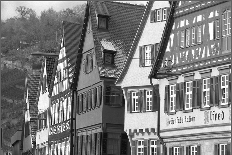
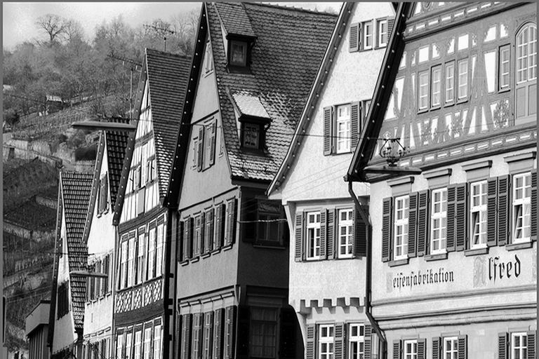
The following example demonstrates the effect of histogram equalization on a grayscale image:

Input Image	Output Image

As shown in the example above, histogram equalization significantly improves the visual quality by redistributing the intensity values across the full dynamic range, making previously hidden details more visible and enhancing overall image contrast.

Algorithm Description#

This algorithm aims to find a new mapping palette based on the histogram. Consider a grayscale image X, whose total number of gray levels in the image is L (\(L=256\) for 8-bit images). Denote the histogram of the image as \(H_x\).

Classical Histogram Equalization Theory#

The theoretical foundation follows these steps:

Probability Distribution: The probability of occurrence of a pixel of level i in the image is:

\[p[i] = \frac{H_x[i]}{N}\]

where \(N\) is total number of pixels in the image
Cumulative Distribution Function (CDF): The cumulative distribution function corresponding to \(p[i]\) is:

\[\operatorname{cdf}_x[i] = \sum_{j=0}^{i} p[j]\]
Intensity Transformation: Using the cumulative distribution function to transform the original pixel value to a new pixel value:

\[y[i] = \operatorname{cdf}_x[i] \times L\]

Practical Implementation Considerations#

The actual implementation modifies the classical algorithm for robustness and performance:

Direct Histogram Computation: Calculate frequency counts directly without probability conversion:

\[H_x[i] = \text{count of pixels with intensity } i\]
Cumulative Histogram: Compute cumulative sums using integer arithmetic:

\[\operatorname{CDF}[i] = \sum_{j=0}^{i} H_x[j]\]
Fixed-Point Implementation: The VPU implementation uses fixed-point arithmetic (with 15-bit precision) for optimal performance. This implementation is realized in the normalize_hist_opt() function which combines minimum value detection, normalization, and lookup table generation:

Minimum Value Detection and Cumulative Distribution:

The algorithm first finds the minimum non-zero cumulative value to prevent contrast compression and computes the full cumulative distribution:

\[\operatorname{CDF}_{\min} = \min\{\operatorname{CDF}[i] : \operatorname{CDF}[i] > 0\}\]

Mathematical Transformation:

The robust intensity transformation applies normalized transformation that handles edge cases:

\[y[i] = \frac{\operatorname{CDF}[i] - \operatorname{CDF}_{\min}}{(M \times N) - \operatorname{CDF}_{\min}} \times 255\]

where \(M \times N\) is the total number of pixels in the image.

Fixed-Point Arithmetic with 15-bit Precision:

The core transformation uses fixed-point arithmetic to maintain precision while optimizing for VPU performance as below:

\[\begin{split}\text{scale} &= \frac{255 \times 2^{15}}{(M \times N) - \operatorname{CDF}_{\min}} \\[0.7em]\end{split}\]

\[\begin{split}\quad\operatorname{normalized\_CDF} &= \operatorname{CDF}[i] - \operatorname{CDF}_{\min} \\[0.7em]\end{split}\]

\[\begin{split}\quad\text{y}[i] &= \mathrm{round}\left(\frac{\operatorname{normalized\_CDF} \times \text{scale}}{2^{15}}\right) \\\end{split}\]

Key Implementation Benefits:
- Numerical Stability: Avoids division by zero when all pixels have the same intensity
- Integer Arithmetic: Eliminates floating-point operations for VPU efficiency
- Proper Contrast Stretching: \(\operatorname{CDF}_{\min}\) normalization ensures full dynamic range utilization
- Fixed-Point Precision: 15-bit scaling maintains accuracy while optimizing performance
Vectorized Pixel Transformation: The final step applies the pre-computed lookup table to transform input pixels using vectorized lookup operations for optimal performance.

Parameters#

Input data type: u8 (8-bit unsigned)
Input format: Single-channel grayscale image
Output data type: u8 (8-bit unsigned)
Data Layout: HWC (Height x Width x Channels)

Implementation Details#

Dataflow Configuration#

The implementation uses three RasterDataFlow (RDF) configurations for efficient data movement and processing:

Source RDF (sourceDataFlow):
- Handles input image tiles with a dedicated trigger (src_trig)
- Essential for histogram computation phase
- Configured with input dimensions and tile size (\(TW \times TH\))
- Uses input_v as tile buffer
Second Source RDF (source2DataFlow):
- Handles second pass of input data with a separate trigger (src_trig2)
- Uses same input dimensions but separate tile buffer (input_v2)
- Essential in histogram equalization phase for pixel remapping
Destination RDF (destinationDataFlow):
- Manages output image tiles with dst_trig trigger
- Uses output_v as tile buffer
- Configured with same tile dimensions as input

Each RDF is configured with tile dimensions of \(384 \times 64\) pixels for optimal performance and uses double buffering to overlap computation and data transfer.

Buffer Allocation#

The implementation requires several VMEM buffers:

Double-buffered input buffers for image tiles
Histogram buffer (\(256\) bins \(\times 32\) vector width)
Normalized histogram buffer (\(256\) bins)
Output buffer for transformed image tiles
Additional buffers for intermediate computations

Kernel Implementation and Vectorization#

The implementation leverages VPU’s vector processing capabilities through three main kernels, each optimized for parallel execution:

Histogram Computation Kernel:
- Uses \(32\)-wide vector operations to process pixels in parallel
- Accumulates frequency counts using vector reduction operations
- Employs vector scatter operations for histogram updates
- Utilizes Address Generators (AGEN) for efficient memory access patterns
- Processes \(32\) pixels per cycle for 8-bit data
Key VPU Instructions Used:

Histogram Computation:
- 32-way Histogram Instruction (vhist_32h): The core VPU histogram instruction that performs weighted histogram accumulation. Takes three parameters:
  - hist: Pointer to the histogram buffer
  - vpix: Pixel values serving as bin indices
  - vweight: Weight vector (set to 1 for simple counting)
  This instruction processes up to 32 histogram updates per cycle, with each pixel value determining which bin to increment.
The implementation uses a simple but efficient approach: for each iteration, pixels are loaded, used as indices for histogram accumulation with unit weights, and results are stored. The chess_unroll_loop(8) directive ensures optimal pipeline utilization by unrolling the inner loop.

Histogram Reduction:
- Vector Addition Operations (vhist.lo + vhist.hi): Combines the low and high parts of the double vector histogram data. This operation consolidates histogram values from different vector lanes to prepare for reduction.
- Vector Sum Reduction (vsumr): Performs horizontal sum reduction across vector elements, accumulating all values within a vector lane into a single sum. This is essential for computing cumulative histogram values across multiple bins.
- Scalar-Vector Addition (vsum + h): Adds scalar histogram values to vector results, enabling the combination of previously computed cumulative sums with current bin contributions for the cumulative distribution function calculation.
The reduction kernel efficiently processes \(niter \times 4\) elements with loop unrolling, combining vector operations with scalar arithmetic to compute the cumulative distribution function required for histogram equalization.
Histogram Normalization Kernel:
- Computes the cumulative sum of histogram bins
- Uses vector min/max operations for histogram boundary computation
- Normalizes using fixed-point arithmetic for performance
- Creates a lookup table for pixel transformation
- Handles edge cases where all pixels have the same intensity
Key VPU Instructions Used:
- Vector Subtraction (v1 - delta): Subtracts the delta value (minimum non-zero histogram value) from all cumulative histogram values. This operation shifts the cumulative distribution to start from zero, which is essential for proper contrast stretching.
- Vector Multiply with Scaling (dvmulwhw): Performs fixed-point multiplication with automatic truncation using VPU_TRUNC_15. This instruction applies the scaling factor \(\frac{255 \times 2^{15}}{(width \times height - delta)}\) to normalize the cumulative values to the output intensity range [0, 255].
- Scalar Loop for CDF Computation: The initial scalar loop computes the cumulative distribution function using hist[i] += i > 0 ? hist[i-1] : 0 and identifies the minimum non-zero value (delta) for normalization.
The normalization kernel efficiently processes \(nbins / vecw\) iterations, transforming cumulative histogram values into a lookup table that maps input pixel intensities to equalized output values using fixed-point arithmetic for optimal VPU performance.
Pixel Transformation Kernel:
- Applies the lookup table using vectorized operations
- Processes multiple pixels in parallel using \(32\)-way SIMD
- Uses efficient vector load/store operations for memory access
- Implements vectorized lookup table operations for final pixel transformation
Key VPU Instructions Used:
- 32-way Vector Lookup (vlookup_32h): The core transformation instruction that applies the lookup table to convert input pixel intensities to equalized output values. Takes two parameters:
  - hist: Pointer to the lookup table created by the normalization kernel
  - vin1/vin2: Input pixel vectors serving as indices into the lookup table
  This instruction performs up to 32 simultaneous lookup operations per call, directly mapping input intensities to their equalized counterparts.
The transformation kernel processes pixels in pairs for maximum efficiency, performing 2 × niter pixel transformations with loop unrolling. Each iteration loads 64 pixels total (\(32 \times 2\)), applies lookup table transformations, and stores the equalized results, achieving optimal throughput for the final histogram equalization stage.

The implementation optimizes performance through:

Vector histogram instructions for parallel bin updates
Address generators for efficient memory access patterns
Double buffering for overlapped data transfer and computation
Optimized Tile size of \(384 \times 64\) pixels for optimal performance
Vector reduction operations for histogram computation
Vector scatter/gather operations for histogram updates

Performance#

Execution Time is the average time required to execute the operator on a single VPU core. Note that each PVA contains two VPU cores, which can operate in parallel to process two streams simultaneously, or reduce execution time by approximately half by splitting the workload between the two cores.

Total Power represents the average total power consumed by the module when the operator is executed concurrently on both VPU cores.

For detailed information on interpreting the performance table below and understanding the benchmarking setup, see Performance Benchmark.

ImageSize	DataType	Execution Time	Submit Latency	Total Power
1920x1080	U8	0.542ms	0.019ms	12.824W