DistanceTransform#
Overview#
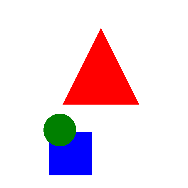
The Distance Transform operator computes the Euclidean distance [1] between each off-pixel (marked as 0xFFFF in this implementation) and the nearest on-pixel (from 0 to 15).
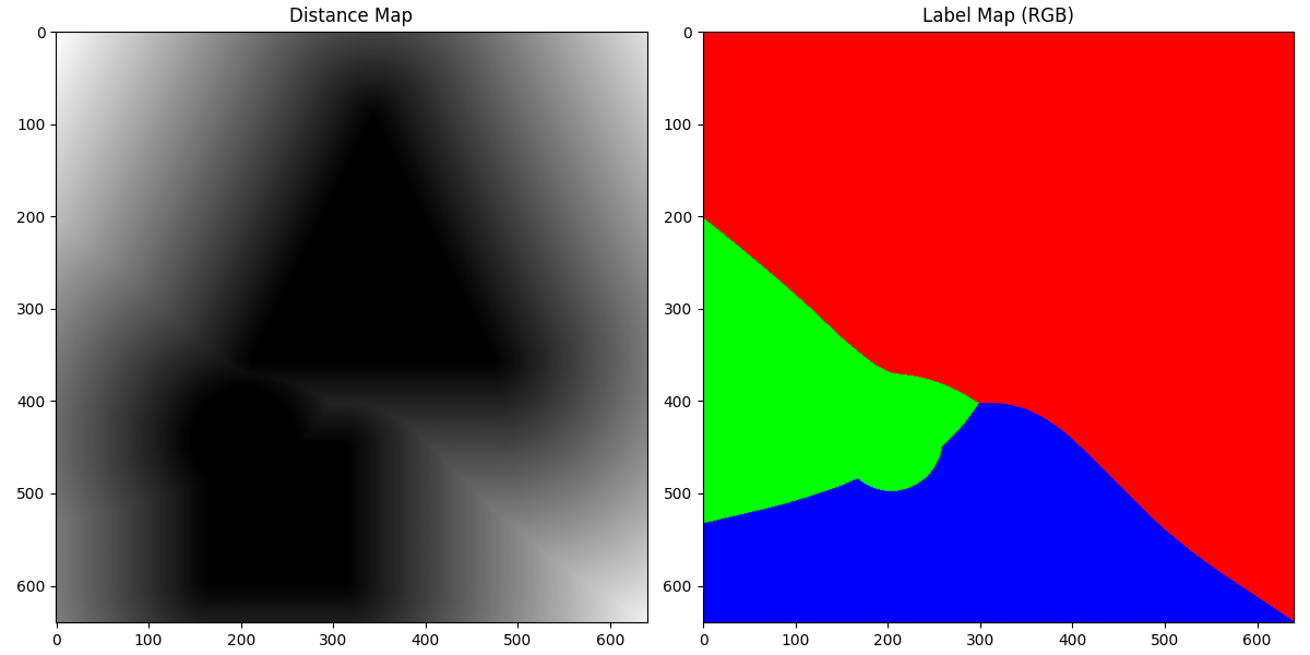
The output is a grayscale image where each pixel’s intensity represents its distance from the nearest on pixel. Higher intensity values indicate pixels that are further.
The distance value is in UQ13.3 format, means the upper 13 bits are integer part and the lower 3 bits are fractional part. For example, 40 means the distance value in float is 40 / 8 = 5.0 pixels.
Another result of the operator is the Voronoi diagram [2] of the input image, which is a pixel-wise label of the nearest on pixel.
The distance transform is typically applied to a binary image, which is a segmented image with unsegmented pixels marked as 0xFFFF and segmented pixels marked as different segment values.
Input Image |
Output Image |
|---|---|
|
|
The labels with the value 0, 1 and 2, are marked as red, green and blue respectively in the voronoi diagram. In the distance result, the brightness shows the distance to from the off pixel to the nearest on pixel.
The operator is particularly useful in:
Shape analysis and pattern recognition
Skeleton extraction
Path planning and obstacle avoidance
Creating distance fields for various computer vision applications
Limitations#
Distance Metric: Supports Euclidean (L2) distance only
Input Format: Requires 16-bit unsigned integer (
U16) input imagesOutput Format: Produces distance maps in
UQ13.3fixed-point format and labels in 8-bit unsigned integer (U8) formatImage Dimensions: Supports image widths and heights between 32 and 1024 pixels
Label Capacity: Can process up to 16 distinct labels in a single image
Implementation Details#
The operator is implemented by vectorizing the algorithm described in the paper “Distance Transforms of Sampled Functions” [3]. The implementation consists of two stages:
A horizontal pass that computes distances along each row independently
A vertical pass that processes the intermediate results to compute final 2D distances
This two-pass approach transforms what would normally be a global optimization problem into two semi-global problems that can be solved independently. By separating the 2D Euclidean distance transform into orthogonal 1D passes, we significantly reduce the computational complexity while still obtaining mathematically exact results. The horizontal pass considers only row-wise distances, while the vertical pass incorporates these results to account for the vertical component of distances.
Stage 1: Horizontal Pass#
Dataflow Configuration#
Two GatherScatterDataFlows are used to load and store the tiles in the horizontal pass.
The reading tile size is set to 32 x image-width rounded up to multiple of 4. For the pixels outside the image boundary, the value is set to 0xFFFF.
The writing tile size is set to 32 x image-width.
The double buffer is used in the horizontal pass.
The computation kernels read from the buffer and in-place write to the buffer so the double buffer are composed of 2 separated buffers in 2 VMEM superbanks.
The RasterDataFlow cannot be used here as the buffer address needs to be alternated in different superbanks.
Vectorization#
There are 2 scan loops in the horizontal pass.
The left-to-right loop starts from the leftmost tile column, transposely reads the pixels, applies the computation as move to the right.
Then the right-to-left loop starts from the rightmost tile column, transposely reads the previous result, applies the computation as move to the left.
In order to save the buffer space, the label and distance are compressed into 16-bit short type by label << 12 | distance.
Stage 2: Vertical Pass#
Dataflow Configuration#
The vertical pass processes tiles in vertical strips, with each tile having dimensions of image-height x 32 pixels.
The implementation uses a single RasterDataFlow for loading input tiles, but requires two separate RasterDataFlows for writing output results.
This split output approach is necessary due to VMEM capacity constraints - the available memory can only accommodate distance and label data for half the image height at a time.
Vectorization#
Similar to the horizontal pass, there are 2 scan loops in the vertical pass.
The top-to-bottom loop starts from the topmost tile row, reads the pixels, applies the computation as move to the bottom.
Then the bottom-to-top loop starts from the bottommost tile row, reads the previous result, applies the computation as move to the top.
The tricky part is there is a while loop in each pass. We compute the stop condition separately in each lane of a vector, mask off the computation of the lanes that have reached the stop condition.
The kernel uses a vandr_s instruction to reduce the stop condition to a single boolean value and the while loop quits when all lanes meet the stop condition.
Performance#
The execution time of the Distance Transform Operator depends on the input data. The profiling results presented in this document are based on the sample image shown above.
Execution Time is the average time required to execute the operator on a single VPU core.
Note that each PVA contains two VPU cores, which can operate in parallel to process two streams simultaneously, or reduce execution time by approximately half by splitting the workload between the two cores.
Total Power represents the average total power consumed by the module when the operator is executed concurrently on both VPU cores.
For detailed information on interpreting the performance table below and understanding the benchmarking setup, see Performance Benchmark.
ImageSize |
Execution Time |
Submit Latency |
Total Power |
|---|---|---|---|
256x256 |
0.435ms |
0.018ms |
10.471W |
1024x1024 |
6.282ms |
0.028ms |
10.27W |