FASTCornerDetector#
Overview#
The Features from Accelerated Segment Test (FAST) algorithm is a widely used method for detecting corners. Its main advantage is low computational complexity. The algorithm’s details can be found in [1], [2], and [3].
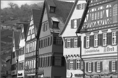
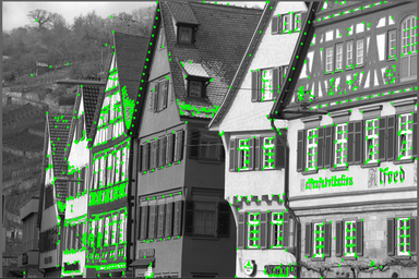
One of the main disadvantages of the FAST corner detector is multiple detections of corners in proximity; therefore, Non-Maximum Suppression (NMS) is often used to refine the output. Since the original algorithm only classifies pixels into corners and non-corners and does not compute a corner response function, NMS cannot be directly applied to the resulting corners. The current implementation follows OpenCV’s approach, which calculates the maximum threshold that makes the target pixel a FAST corner and uses this threshold (called the score) as the input for NMS. More details can be found in [4]. Other methods to calculate scores, such as computing the sum of absolute differences between surrounding pixels and center pixels, are also available in the literature. The sample input image and output results are shown in the following figures, where the green dots are the detected corners.
|
|
Figure 1: Sample input image (left) and output results (right). Data type is uint16_t, threshold is 15428 and NMS is ON.
Design Requirements#
Data type supports
uint8_t,uint16_t,int8_tandint16_t.Supports a circle radius of 3 and an arc length of 9.
NMS can be ON or OFF.
The output location is X-Y interleaved float. Note that the order of locations is implementation-specific; additional sorting may be needed to compare locations from different implementations.
The image border extension type can be constant or replicate.
Implementation Details#
Quick Rejection#
To further reduce computational complexity, a quick rejection method is adopted. This method conducts an initial test to eliminate pixels that are not corners, allowing only non-rejected pixels to undergo further testing and score calculation if they are corners. The quick rejection method described in “High-speed test” of [2] refers to a configuration with a circle radius of 3 and an arc length of 12.
The proposed scheme tests pixel P1, P5, P9, and P13 (shown in the following figure) and rejects the central pixel if at least three of their intensities are within the range \([I_{p}-t, I_{p}+t]\), where \(I_{p}\) is the central pixel’s intensity and \(t\) is the threshold. This scheme has a lower rejection ratio compared to that in “High-speed test” of [2]. For an arc length of 9, it is possible for a candidate pixel to be a corner even if only 2 out of 4 testing pixels are both brighter than \(I_{p}+t\) or darker than \(I_{p}-t\). As the current implementation uses SIMD instructions to process 1x32 pixels as a chunk, it is also necessary to test a contiguous block of 1x32 pixels and reject them as a whole if all satisfy the rejection criteria. In other words, if there is even one pixel that does not meet the rejection criteria, this 1x32 pixel chunk will not be rejected.
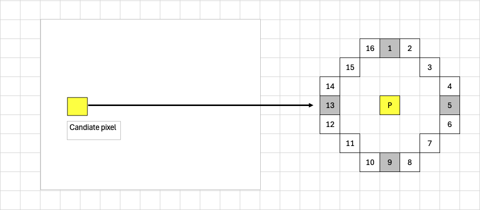
Figure 2: Quick Rejection Illustration#
The rationale behind quick rejection is that corners are quite sparse in practical scenarios, e.g., less than 1% of the image’s total pixels. The time consumption after adopting quick rejection becomes
quick_rejection_time + non_rejection_ratio * score_calculation_time, leading to two implications:
If
quick_rejection_timeis smaller thanscore_calculation_time, overall time consumption will be reduced using quick rejection whennon_rejection_ratiois small.In rare cases where
non_rejection_ratiois relatively large (e.g., 10%), overall time consumption may increase compared to not using quick rejection.
Dataflow Configuration#
1. Use RDF dataflow to transfer tiles from DRAM to VMEM, similar to a 7x7 2D filtering process. For each tile, calculate scores and transfer them back from VMEM to DRAM as a height * width image in tight
layout, with values representing scores. This step prepares for overlapping tiles required by NMS.
2. Use RDF dataflow again to transfer the score-valued image from DRAM to VMEM, akin to a 3x3 2D filtering operation. For each tile, perform NMS; for each non-zero NMS output, calculate its location within the entire image and output it in X-Y interleaved format. SQDF dataflow transfers these locations from VMEM to DRAM. The number of locations varies among tiles, necessitating a similar mechanism to maintain related states on both device and host sides. More information can be found in the documentation regarding the MinMaxLoc operator’s output.
When NMS is OFF, the above two steps can be merged into one step. In this case, the scores do not need to be transferred back to DRAM, as the locations can be directly calculated based on the scores. The host code uses flags to set up different dataflows. The device code uses separately built binaries for NMS being either ON or OFF to avoid branches in the device code.
Different Data Types Support#
The support for different data types has several implications:
1. From the algorithm’s perspective, the score result is always larger than or equal to 0 since the current corner response function uses the absolute difference between the central pixel and the surrounding
pixels. Although the final output is float type, the intermediate representation always uses int16_t type. This is independent of the data type of the score, since otherwise uint8_t type can only support a maximum coordinate value of 255.
2. From the VPU implementation’s perspective, the PVA hardware constraint requires that double vector load/store must be 2-byte-aligned. Therefore, two single byte-type vector load instructions must be used to populate a double vector of byte type if an address is 1-byte-aligned.
3. From the performance perspective, when comparing the implementation of signed and unsigned types, the device code only differs in the variants of the load and store instructions used (e.g., vuchar_load
versus vchar_load), which has no performance impact. Additionally, the support for different data types has been separately built into different device code binaries to avoid branch penalties. Combined with NMS options, this results in a total of 8 different device code binaries.
Performance#
Execution Time is the average time required to execute the operator on a single VPU core.
Note that each PVA contains two VPU cores, which can operate in parallel to process two streams simultaneously, or reduce execution time by approximately half by splitting the workload between the two cores.
Total Power represents the average total power consumed by the module when the operator is executed concurrently on both VPU cores.
For detailed information on interpreting the performance table below and understanding the benchmarking setup, see Performance Benchmark.
ImageSize |
DataType |
TestData |
Execution Time |
Submit Latency |
Total Power |
|---|---|---|---|---|---|
1024x1024 |
U8 |
Random |
1.685ms |
0.017ms |
11.72W |
1920x1080 |
U8 |
Random |
3.324ms |
0.018ms |
11.336W |
1920x1080 |
U8 |
kodim08_grayscale_1920x1080_u16 |
1.799ms |
0.018ms |
11.738W |
1024x1024 |
U16 |
Random |
2.883ms |
0.018ms |
11.82W |
1920x1080 |
U16 |
Random |
5.684ms |
0.019ms |
11.82W |
1920x1080 |
U16 |
kodim08_grayscale_1920x1080_u16 |
3.598ms |
0.018ms |
11.638W |
Note: For performance measurements using real images, the uint8_t data type case uses the same source image as the uint16_t case. During image loading, the data is converted from uint16_t to uint8_t on the fly, ensuring both cases operate on identical image content.