Intro to Calibration | AODT Documentation

1. Introduction

Calibration closes the gap between a clean simulation and a measured real-world site. It uses field measurements from one campaign to tune the scene model, so later simulations of that same environment start from behaviour that has already been anchored to reality instead of relying only on default assumptions.

Under the hood, the electromagnetic (EM) engine — ray tracing plus EM field computation (see the EM physics primer) — stays fixed as the forward model; calibration adjusts its inputs (chiefly the materials, and optionally other set-up quantities such as antenna orientations and beams — see Calibration targets) until the engine’s predictions match the measurements.

Calibration is always done from an environment and for that same environment.

This tie to a single scene is fundamental: the materials describe the exact place that was measured and hold only within that same geometry, so the same scenario is required throughout — materials calibrated in one place cannot be applied to another.

End to end, calibration is a four-step loop; the rest of the guide refers back to these steps:

Measurement campaign — the actual, real-world field measurements must be provided as input; the tool never synthesizes them, so calibration is only as good as the real data supplied:
- GPS Exchange Format (GPX) trace of the User Equipment (UE) positions
- A power-level trace per Radio Unit (RU)–UE link — not a single number, but a series of power values sampled along the UE trajectory (one CSV file per link)
Aligned simulation in AODT — reproduce the campaign synthetically:
- Match the real scenario on map and georeferencing
- Ensure frequency settings, RU locations, and UE locations are accurately set
- See Simulation setup
Calibration — combine the rays exported in the simulation with the measurements from step 1:
- The main outputs are the material categories of the campaign environment: calibrated building-material outputs and, when vegetation is present and hit by rays, calibrated vegetation-material outputs
- See Calibration and Training
Post-processing simulations — reuse the recovered calibrated building-material outputs and calibrated vegetation-material outputs:
- Generalize any other simulation in that same environment
- See Post-processing

Calibration is a model-based inverse problem, not a black-box curve fit. The physics EM engine stays fixed as the forward model: it traces rays through the scene, applies material-dependent reflection, transmission, diffraction, and scattering effects, and predicts the received power at each link. Calibration runs that relationship backwards:

Disclaimer: calibration is in an early alpha version and has not yet been tested extensively enough to guarantee results. Treat every output as experimental and validate it against held-out measurements before relying on it.

The main practical boundaries are maintained in Calibration limitations, including data knowledge, generalization, and recoverability limits.

Simple calibration file bundle

Use this bundle as a quick lookup for the files a calibration campaign needs. The paths are intentionally general-purpose: replace path/to/campaign/ with the folder or object-store prefix used by the run.

Files needed:

one GPX trace excerpt of the UE route — to learn more, see §2.1 UEs
two Reference Signal Received Power (RSRP) measurement CSV excerpts under measurements/ — to learn more, see §3.2 Power measurements
no map files in the bundle; the scene and optional vegetation are referenced by location

campaign/

sim.yml

1 db:
2   db_author: aerial
3   db_host: clickhouse
4   db_port: 9000
5   opt_in_tables:
6   - cfrs
7   - raypaths
8   - cirs
9   opt_in_tables_options:
10     raypaths: full
11   parquet_export:
12     compression: zstd
13     iceberg:
14       catalog_name: default
15       catalog_type: rest
16       catalog_uri: https://iceberg-catalog.example.com/
17       nessie_ref: main
18       database: simple_campaign_input
19     max_workers: 2
20     s3_configs:
21     - access_key: STORAGE_ACCESS_KEY
22       bucket: my-calibration-bucket
23       endpoint_url: https://object-store.example.com
24       nodes:
25       - node1
26       provider: minio
27       region: us-east-1
28       secret_key: STORAGE_SECRET_KEY
29       use_ssl: false
30     timesteps_per_file: 100
31     verify_exports: true
32   sim_id: simple_campaign_input
33   s3_config:
34     bucket: my-calibration-bucket
35     endpoint_url: https://object-store.example.com
36     access_key: STORAGE_ACCESS_KEY
37     secret_key: STORAGE_SECRET_KEY
38     provider: minio
39     region: us-east-1
40 gis:
41   scene:
42     scene_url: my_scene
43   spawn_zone:
44     points_ccw:
45     - x: -100.0
46       'y': -100.0
47     - x: 100.0
48       'y': -100.0
49     - x: 100.0
50       'y': 100.0
51     - x: -100.0
52       'y': 100.0
53   vegetation:
54     active: true
55     geojson:
56     - path/to/campaign/vegetation.geojson
57     vegetation_asset_path:
58     - path/to/assets/street_tree.json
59 sim:
60   DUs:
61     add:
62     - id: 1
63       position:
64         pos:
65           x: 0.0
66           'y': 0.0
67           z: 0.0
68     default: path/to/assets/du.json
69     update:
70     - attributes:
71         aerial_du_fft_size: 1
72         aerial_du_max_channel_bandwidth: 100.0
73         aerial_du_num_antennas: 1
74         aerial_du_reference_freq: 3619.0
75         aerial_du_subcarrier_spacing: 60.0
76       ids:
77       - 1
78   Materials:
79     default: path/to/assets/materials.json
80   Panels:
81     add:
82     - id: 1
83     - id: 2
84     default: path/to/assets/panel.json
85     update:
86     - attributes:
87         antenna_names:
88         - halfwave_dipole
89         antenna_roll_angle_first_polz_degree: 0.0
90         antenna_roll_angle_second_polz_degree: 90.0
91         antenna_spacing_horz_mm: 41.419239845261124
92         antenna_spacing_vert_mm: 41.419239845261124
93         dual_polarized: false
94         num_loc_antenna_horz: 1
95         num_loc_antenna_vert: 1
96         reference_freq_mhz: 3619.0
97       ids:
98       - 1
99     - attributes:
100         antenna_names:
101         - threeGPP_38901
102         antenna_roll_angle_first_polz_degree: 0.0
103         antenna_roll_angle_second_polz_degree: 90.0
104         antenna_spacing_horz_mm: 41.419239845261124
105         antenna_spacing_vert_mm: 41.419239845261124
106         dual_polarized: false
107         num_loc_antenna_horz: 1
108         num_loc_antenna_vert: 1
109         reference_freq_mhz: 3619.0
110       ids:
111       - 2
112   RUs:
113     add:
114     - id: 2
115       position:
116         pos:
117           x: 3420.0
118           'y': 3980.0
119           z: 3025.0
120     - id: 1
121       position:
122         pos:
123           x: -13390.0
124           'y': -4090.0
125           z: 3275.0
126     default: path/to/assets/gnb.json
127     update:
128     - attributes:
129         aerial_gnb_carrier_freq: 3619.0
130         aerial_gnb_du_id: 1
131         aerial_gnb_du_manual_assign: true
132         aerial_gnb_height: 1.5
133         aerial_gnb_mech_azimuth: 195.0
134         aerial_gnb_mech_tilt: 5.0
135         aerial_gnb_panel_type: 2
136         aerial_gnb_radiated_power: 43.0
137       ids:
138       - 2
139     - attributes:
140         aerial_gnb_carrier_freq: 3619.0
141         aerial_gnb_du_id: 1
142         aerial_gnb_du_manual_assign: true
143         aerial_gnb_height: 1.5
144         aerial_gnb_mech_azimuth: 280.0
145         aerial_gnb_mech_tilt: 5.0
146         aerial_gnb_panel_type: 2
147         aerial_gnb_radiated_power: 43.0
148       ids:
149       - 1
150   Scatterers:
151     default: path/to/assets/car_small.json
152   Scenario:
153     default: path/to/assets/scenario.json
154     update:
155     - attributes:
156         sim_batches: 1
157         sim_duration: 1.0
158         sim_em_diffuse_type: 0
159         sim_em_interactions: 5
160         sim_em_max_num_paths_per_ant_pair: 500
161         sim_em_rays: 1000
162         sim_enable_wideband: true
163         sim_gnb_panel_type: 2
164         sim_interval: 0.51
165         sim_is_full: false
166         sim_is_seeded: true
167         sim_samples_per_slot: 1
168         sim_seed: 42
169         sim_simulation_mode: 0
170         sim_slots_per_batch: 0
171         sim_ue_panel_type: 1
172         sim_ue_min_speed: 1.5
173         sim_ue_max_speed: 1.5
174   UEs:
175     add:
176     - gpx:
177         src: path/to/campaign/gpx/route_10.gpx
178         use_pathfinding: false
179       id: 1
180     default: path/to/assets/ue.json
181     update:
182     - attributes:
183         aerial_ue_bler_target: 0.1
184         aerial_ue_initial_mech_azimuth: 0.0
185         aerial_ue_manual: true
186         aerial_ue_mech_tilt: 0.0
187         aerial_ue_panel_type: 1
188         aerial_ue_radiated_power: 26.0
189       ids:
190       - 1
191     - attributes:
192         aerial_ue_radiated_power: 26.0
193       ids:
194       - '*'
195   VegetationMaterials:
196     default: path/to/assets/vegetation_materials.json
197   BldgExterior:
198     update:
199     - attributes:
200         AerialRFDiffraction: true
201         AerialRFDiffuse: true
202         AerialRFMesh: true
203         AerialRFTransmission: true
204         AerialRFdS: 15.0
205       ids:
206       - '*'

cal.yml

The db:, gis:, and sim: blocks are the same as in sim.yml above and are omitted here. Only the calibration-specific cal: block is shown.

1 # db:, gis:, and sim: — same as sim.yml (omitted)
2 cal:
3   targets:
4     Materials: true
5     VegMaterials: false
6     UEs: true
7     RUs: true
8     RUsBeams: false
9   timeline:
10     start: 0
11     step: 1
12     end: 9
13   measurements:
14   - ru_id: 1
15     ue_id: 1
16     measurement_file: path/to/campaign/measurements/ru1_ue1_rsrp.csv
17   - ru_id: 2
18     ue_id: 1
19     measurement_file: path/to/campaign/measurements/ru2_ue1_rsrp.csv
20   output:
21     folder_key: path/to/calibrated-output/simple-campaign/

gpx/route_10.gpx

1 <?xml version="1.0" encoding="UTF-8"?>
2 <gpx version="1.1" xmlns="http://www.topografix.com/GPX/1/1"
3      xmlns:xsi="http://www.w3.org/2001/XMLSchema-instance"
4      xsi:schemaLocation="http://www.topografix.com/GPX/1/1 http://www.topografix.com/GPX/1/1/gpx.xsd">
5   <metadata>
6     <name>Helsinki Route (10 samples)</name>
7     <desc>10-point excerpt, Helsinki</desc>
8   </metadata>
9   <trk>
10     <name>Helsinki Route</name>
11     <trkseg>
12       <trkpt lat="60.1708822852" lon="24.9359953119">
13         <ele>8.596870</ele>
14         <time>2024-06-15T10:00:00Z</time>
15       </trkpt>
16       <trkpt lat="60.1708739291" lon="24.9359748632">
17         <ele>8.618520</ele>
18         <time>2024-06-15T10:00:01Z</time>
19       </trkpt>
20       <trkpt lat="60.1708655730" lon="24.9359544145">
21         <ele>8.640169</ele>
22         <time>2024-06-15T10:00:02Z</time>
23       </trkpt>
24       <trkpt lat="60.1708572169" lon="24.9359339658">
25         <ele>8.661819</ele>
26         <time>2024-06-15T10:00:04Z</time>
27       </trkpt>
28       <trkpt lat="60.1708488608" lon="24.9359135171">
29         <ele>8.683468</ele>
30         <time>2024-06-15T10:00:05Z</time>
31       </trkpt>
32       <trkpt lat="60.1708405047" lon="24.9358930684">
33         <ele>8.705117</ele>
34         <time>2024-06-15T10:00:07Z</time>
35       </trkpt>
36       <trkpt lat="60.1708321486" lon="24.9358726197">
37         <ele>8.726767</ele>
38         <time>2024-06-15T10:00:08Z</time>
39       </trkpt>
40       <trkpt lat="60.1708237925" lon="24.9358521710">
41         <ele>8.748416</ele>
42         <time>2024-06-15T10:00:10Z</time>
43       </trkpt>
44       <trkpt lat="60.1708154363" lon="24.9358317223">
45         <ele>8.770065</ele>
46         <time>2024-06-15T10:00:11Z</time>
47       </trkpt>
48       <trkpt lat="60.1708070802" lon="24.9358112736">
49         <ele>8.791715</ele>
50         <time>2024-06-15T10:00:13Z</time>
51       </trkpt>
52     </trkseg>
53   </trk>
54 </gpx>

For more information about the GPX trace and UE setup, see §2.1 UEs.

measurements/ru1_ue1_rsrp.csv

1 uniqtimestamp,time,Power_PCI_1
2 ,0,-80.10551452636719
3 ,1,-78.56816101074219
4 ,2,-78.04997253417969
5 ,3,-76.04109954833984
6 ,4,-77.53031921386719
7 ,5,-80.73326873779297
8 ,6,-83.16703033447266
9 ,7,-83.58888244628906
10 ,8,-84.93547058105469
11 ,9,-84.13796997070312

For more information about power measurements, see §3.2 Power measurements.

measurements/ru2_ue1_rsrp.csv

1 uniqtimestamp,time,Power_PCI_2
2 ,0,-54.06867980957031
3 ,1,nan
4 ,2,-51.98063278198242
5 ,3,nan
6 ,4,nan
7 ,5,-53.42338943481445
8 ,6,-56.82176971435547
9 ,7,-61.351783752441406
10 ,8,-59.29664993286133
11 ,9,-56.15536117553711

For more information about power measurements, see §3.2 Power measurements.

2. Simulation setup

Goal. Before calibration starts, reproduce the measurement campaign inside AODT so the traced rays and real measurements describe the same links. Match the configuration that determines:

map georeferencing
link geometry (§2.1 UE placement and §2.2 RU placement)
antenna setup
scene RF interactions
frequency settings

This setup belongs to the simulation that precedes calibration. The fields here become the fixed context for the following calibration pass, which relies on the rays, links, and frequency samples produced by that previous simulation. This connects directly to Calibration targets and §4 Outputs.

How this section is organized. Each category below uses the same layout:

Configuration snippet — YAML fields that the following calibration step will rely on for that category.
Using existing campaign data — if campaign data is already available (GPX traces, mounting angles, antenna patterns, site coordinates, and so on) and do not need the full background, map the user’s inputs onto the snippet fields wherever possible. The more accurate the values supplied here, the less ambiguity the following calibration step has to resolve.
Limitations — hard constraints and common mistakes for that category.

For each target, §3.3 Calibration targets summarizes which quantities are optimized and which remain fixed.

Categories covered: §2.1 UEs, §2.2 RUs, §2.3 Scenario, §2.4 Frequency. For the material-category flow, the key setup checks are scene RF interactions and frequency settings.

2.1 UEs

In this section, a UE calibration target means a UE from the measured campaign that can be part of one or more targeted RU-UE links. The same UE can appear in multiple targeted links, for example when several RUs measured the same UE route. The following calibration step uses measurements on those links to compare the EM prediction against the campaign data. From that UE, calibration can later recover the device orientation along the route — its tilt, its azimuth, and the panel roll — while the GPX position is always kept exactly as measured (full detail in §3.3 UEs). The fields below are the setup inputs that feed that step.

Configuration snippet

Calibration-relevant UE and linked panel settings:

1 sim:
2   UEs:
3     add:
4       - id: 1
5         gpx:
6           src: path/to/route.gpx  # a UE calibration target must be defined from a GPX file
7           use_pathfinding: false
8     update:
9       - ids:
10           - 1
11         attributes:
12           aerial_ue_panel_type: 3  # Links the UE to panel id 3; training details in §3.3 UEs
13           aerial_ue_mech_tilt: 39.9414128887659  # Setup value; training details in §3.3 UEs
14           aerial_ue_initial_mech_azimuth: 0.0  # Not learnable; imported setup value
15   Panels:
16     update:
17       - ids:
18           - 3
19         attributes:
20           num_loc_antenna_horz: 1  # Important: keep antennas as single element
21           num_loc_antenna_vert: 1  # Important: keep antennas as single element
22           dual_polarized: false
23           antenna_names: [halfwave_dipole]  # built-in name or polarimetric CSV/FFD path
24           antenna_roll_angle_first_polz_degree: 0.0  # Setup value; training details in §3.3 UEs
25           antenna_roll_angle_second_polz_degree: 90.0  # Setup value; training details in §3.3 UEs

This snippet only identifies the UE setup values used by the UE calibration target.

The full trained / not-trained split is described in §3.3 UEs.

Using existing campaign data

Panel link — aerial_ue_panel_type selects which Panels block describes the UE antenna (3 → panel id 3); the value must match an id under Panels.
Roll emits a new panel — learning the UE panel roll writes a new per-UE panel rather than editing the base block (see §3.3 UEs).
GPX trajectory — set gpx.src to the recorded route file. Each <trkpt> supplies lat, lon, and elevation for one sample:

route.gpx

1 <trkpt lat="60.1708321486" lon="24.9358726197">
2   <ele>8.726767</ele>
3   <!-- optional — per-time-index ue_tilt / ue_azimuth; see below -->
4   <extensions>
5     <angles>
6       <ue_tilt>0.0</ue_tilt>
7       <ue_azimuth>0.0</ue_azimuth>
8     </angles>
9   </extensions>
10 </trkpt>
11 <trkpt lat="60.1708237925" lon="24.9358521710">
12   <ele>8.748416</ele>
13 </trkpt>

Per-time-index UE angles must be supplied through GPX — when per-sample UE orientation is known, provide it on each <trkpt> in the <extensions> block (the same format written by calibration output — see §4 UE GPX output). Section §3.3 UEs explains how these GPX values relate to the trained UE terms. Values that can be supplied per time index:
- ue_tilt — the tilt for that sample
- ue_azimuth — the azimuth for that sample
Antenna pattern — to set up UE antenna types on the panel selected by aerial_ue_panel_type, use one of:
- Custom pattern — supply a custom pattern file path; see Panel.create_panel_from_file.
- Built-in pattern — select a built-in pattern constant; see Panel.create_panel.
Panel geometry — keep the UE panel as a single element:
- num_loc_antenna_horz: 1
- num_loc_antenna_vert: 1
- roll angles — supply as starting values if known.

Limitations

UE setup constraints are consolidated under Calibration limitations → Simulation before calibration → UEs.

2.2 RUs

In this section, an RU calibration target means an RU from the measured campaign that belongs to a targeted RU-UE link. The current calibration ingestion supports one UE only, so the same RU cannot appear in multiple RU-UE links. The following calibration step uses measurements on that link to compare the EM prediction against the campaign data. From that RU, calibration can later recover its mounting orientation and panel roll, while the RU position and height should already match the campaign as closely as possible. The fields below are the setup inputs that anchor every traced link.

Configuration snippet

Calibration-relevant RU and linked panel settings:

1 sim:
2   RUs:
3     add:
4       - id: 1
5         position:
6           pos:
7             x: -13390.0
8             y: -4090.0
9             z: 3275.0
10     update:
11       - ids:
12           - 1
13         attributes:
14           aerial_gnb_height: 1.5  # meters — see effective-z formula below
15           aerial_gnb_panel_type: 4  # Learnable feature through panel roll
16           aerial_gnb_mech_azimuth: 0.031  # Learnable feature (seed)
17           aerial_gnb_mech_tilt: 39.21  # Learnable feature (seed)
18   Panels:
19     update:
20       - ids:
21           - 4
22         attributes:
23           antenna_names: [threeGPP_38901]
24           num_loc_antenna_horz: 1  # Single element so the ray launch sits at the panel phase center (see two-stage note in §2.2)
25           num_loc_antenna_vert: 1  # Multi-element here would offset the launch point and misalign the beam array factor
26           dual_polarized: false
27           antenna_roll_angle_first_polz_degree: -22.75  # Learnable roll angle
28           antenna_roll_angle_second_polz_degree: 67.25  # Learnable roll angle

Using existing campaign data

Calibration reuses the same panel inputs as any AODT custom panel — no calibration-specific antenna file format. Map the site data directly:

Panel link — aerial_gnb_panel_type selects which Panels block describes the RU antenna (4 → panel id 4); the value must match an id under Panels.
Roll is the learnable part — the roll angles on that block (antenna_roll_angle_first_polz_degree / antenna_roll_angle_second_polz_degree) are what calibration trains.
A new panel is emitted, not edited in place — the input panel is only the base; when RU orientation is calibrated, the recovered roll is written as a new panel for that RU, identical to the input but with rotated roll (see §3.3 RUs and §4 Calibrated simulation configuration).
Single-polarized, two roll angles — dual_polarized: false is kept on both input and output, but the estimate is computed under the hood as a combination of two polarizations, so two roll angles appear even though the panel is single-polarized.
3D location — place the RU with one of the supported position inputs:
- Georeferenced latitude/longitude — same as the Config API Position.georef(lat, lon, alt) path; the YAML loader accepts lat / lon under position.pos.
- Cartesian coordinates — set position.pos as (x, y, z) on the georeferenced map.
Antenna height — set aerial_gnb_height (meters). The traced antenna reference is not position.pos.z alone. The effective antenna z uses:
- meters_per_unit — map-specific scale factor (default 0.01; see EM solver API)
- z — RU position.pos.z
- aerial_gnb_height — RU antenna height in meters
The final z coordinate is:
$z_\text{antenna} = z + \frac{h / \text{meters\_per\_unit}}{2}$
Example: with meters_per_unit: 0.01, z: 3275, and aerial_gnb_height: 1.5, the final z coordinate is 3275 + (1.5 / 0.01) / 2 = 3350.
Mounting angles — set the best available survey or installation values:
- aerial_gnb_mech_azimuth
- aerial_gnb_mech_tilt
Antenna pattern — to set up RU antenna types on the panel selected by aerial_gnb_panel_type, use one of:
- Custom pattern — supply a custom pattern file path; see Panel.create_panel_from_file.
- Built-in pattern — select a built-in pattern constant; see Panel.create_panel.

Panel geometry uses two stages — this separates ray tracing from the EM/beam computation. The simulation that exports ray paths uses a single-element RU panel: with one element the ray launch/arrival point sits exactly at the panel phase center, so the traced geometry and the later beam array factor share the same origin. Beam calibration then uses a separate multi-element panel in the calibration/follow-up config; that array defines the beamforming degrees of freedom (the array factor) and is reflected in the §4 Outputs.

If the simulation panel is not single-element, the per-element launch points are offset from the panel center, the beam array factor applied during calibration is misaligned with the traced geometry, and the resulting beam predictions are not guaranteed. Conversely, a single-element panel in calibration has no array factor at all, so no beams can be recovered — beam calibration is only possible on the multi-element array.

Simulation input: ray paths

1 sim:
2   RUs:
3     update:
4     - ids: [1]
5       attributes:
6         aerial_gnb_panel_type: 4
7   Panels:
8     update:
9     - ids: [4]
10       attributes:
11         antenna_names: [threeGPP_38901]
12         num_loc_antenna_horz: 1
13         num_loc_antenna_vert: 1

Calibration/follow-up: beams

1 sim:
2   RUs:
3     update:
4     - ids: [1]
5       attributes:
6         aerial_gnb_panel_type: 4
7   Panels:
8     update:
9     - ids: [4]
10       attributes:
11         antenna_names: [threeGPP_38901, threeGPP_38901, threeGPP_38901, threeGPP_38901]
12         num_loc_antenna_horz: 1
13         num_loc_antenna_vert: 4

See §3.3 RUsBeams for how to size the calibration array.

Limitations

RU setup constraints are consolidated under Calibration limitations → Simulation before calibration → RUs.

2.3 Scenario

The scene geometry only participates in propagation once its RF behaviour is switched on. These switches decide which paths the ray tracer can generate — and therefore which interactions calibration can later attribute to a material.

Configuration snippet

1 sim:
2   BldgExterior:
3     update:
4     - attributes:
5         AerialRFMesh: true          # reflection
6         AerialRFTransmission: true  # transmission — DEFAULT IS false
7         AerialRFDiffuse: true       # diffuse scattering
8         AerialRFdS: 15.0            # scattering surface-element area
9         AerialRFDiffraction: true   # diffraction
10       ids:
11       - '*'
12 
13 gis:
14   vegetation:
15     active: true   # vegetation is OFF by default — must be turned on
16     geojson:
17     - path/to/vegetation.geojson
18     vegetation_asset_path:
19     - path/to/assets/street_tree.json

Limitations

Scene RF-interaction constraints are consolidated under Calibration limitations → Simulation before calibration → Materials and scenario; the GIS / vegetation-setup constraints are under Calibration limitations → Simulation before calibration → Vegetation materials.

Choosing AerialRFdS (scattering element area ds). ds is the area $\Delta S$ each facade is tiled into; one scattered ray launches per element (see Surface diffuse scattering).

Large ds — fewer surface elements and lower ray cost, but sparse scattering hits can leave weak or vanishing gradients during training.
Small ds — finer scattering coverage and stronger calibration signal, but it burns the ray budget.

2.4 DU frequency settings

Calibration is narrowband by design: one campaign constrains materials at a single center frequency. Cross-frequency generalization requires repeating the campaign at another center frequency (see Introduction); the material terms affected by this narrowband assumption are summarized under §3.3 Materials calibration target.

Configuration snippet

Select the DU FFT size to match how the campaign was measured:

1 sim:
2   DUs:
3     update:
4     - attributes:
5         aerial_du_fft_size: 512   # in-band RSRP — use 1 for out-of-band single carrier

Set the carrier on each RU to match the campaign:

1 sim:
2   RUs:
3     update:
4     - ids: [1]
5       attributes:
6         aerial_gnb_carrier_freq: 3619.0

Using existing campaign data

Map the measurement setup directly:

Know the campaign type — set aerial_du_fft_size from the measurement modality:
- Out-of-band single-tone — use aerial_du_fft_size: 1 for one frequency sample per ray.
- In-band RSRP — use aerial_du_fft_size: 512 so power is assessed over the 20 lowest PRBs from the narrowband CFR.
Carrier frequency — set aerial_gnb_carrier_freq on each RU to the center frequency used when the power CSVs were collected.

Limitations

Frequency-setting constraints are consolidated under Calibration limitations → Simulation before calibration → General.

2.5 Unsupported or ignored settings

Some simulation features are useful in other AODT workflows but should not be treated as calibration inputs.

Unsupported / ignored-setting constraints are consolidated under Calibration limitations → Simulation before calibration → General.

3. Calibration

Simulation setup produced the first required input for the following calibration run: the aligned AODT simulation with its traced rays. Calibration also requires the per-link power measurements from the real campaign (§3.2 Power measurements).

This section is the run that combines the imported rays from the previous simulation with those measurements and solves the inverse problem — holding the observed power fixed and recovering the materials that best explain it (see the inverse arrow in Introduction).

A run is driven by a single calibration config with two halves: a db: block that imports the prior simulation (3.1) and a cal: block that defines the job (3.4), which is then optimized during training.

3.1 Importing from the previous simulation

Calibration does not re-trace the scene. The geometry is fixed and only the materials are unknown, so the rays exported by the aligned AODT simulation are read back as the geometric backbone of the forward model. The db: block points the run at that simulation’s database:

1 db:
2   sim_id: my_aligned_campaign   # the simulation to import
3   opt_in_tables:
4   - cfrs          # Optional
5   - raypaths      # Required
6   - cirs          # Optional
7   opt_in_tables_options:
8     raypaths: first              # first-antenna only per-path geometry, not just summaries

sim_id selects the prior simulation to import — this is the import.
opt_in_tables pulls the traced quantities calibration consumes: the per-path raypaths (with raypaths: first), and the cfrs / cirs derived from them.

There is only one traced realization per path for each RU–UE link, paired with that link’s measurements in 3.4.

The imported simulation must be the aligned one. Calibration recovers materials for the exact geometry it imports. If the rays come from a scene that does not match the real campaign (map, georeferencing, RU/UE positions, frequency), the recovered materials are meaningless (see Introduction).

3.2 Power measurements

Accurate signal or per-path knowledge is impractical to collect at larger scale: it usually requires experts and specialized equipment, and does not align with the in-band, widely available, simple measurements most deployments can actually capture. For this reason, the choice uses power as the reference quantity for calibration.

Each measurement is a simple CSV, one file per RU–UE link and one PCI per file. Do not place multiple Power_PCI_<n> columns in the same measurement file. The columns matter more than the row count:

time — sample (time-step) index along the campaign
Power_PCI_<n> — measured power level (RSRP, dBm) for the Physical Cell Identity (PCI) n
beam_idx_PCI_<n> — optional index of the active beam for PCI n at that sample; omit it when the campaign has no beams

template_measurements.csv

1 time, Power_PCI_1, beam_idx_PCI_1   # beam_idx_PCI_1 is OPTIONAL
2 0,   -80.106,      1
3 1,   -78.568,      3

Measurements are attached to the calibration config per link — one CSV per RU–UE pair. That wiring is covered in §3.4 Measurements — per-link inputs under the calibration run.

Checks before calibration:

Make sure all measurement files match the same file format (same columns and layout).
Keep exactly one Power_PCI_<n> column, and optionally its matching beam_idx_PCI_<n> column, per file.
In the absence of beams, calibration cannot estimate any beam.
Every nan or invalid power level is skipped.

Power-measurement constraints are consolidated under Calibration limitations → Calibration process → Power measurements and training.

3.3 Calibration targets

cal.targets is a set of per-quantity switches. Only the targets set to true are trained and become the unknowns that receive gradient updates during training; everything left false is held fixed at the values imported from the simulation database. Each enabled target maps to an artifact in §4 Outputs.

1 cal:
2   targets:
3     Materials:    true       # building / surface materials
4     VegMaterials: true       # vegetation materials
5     UEs:          true       # UE orientation (tilt, azimuth, panel roll)
6     RUs:          true       # radio-unit set-up
7     RUsBeams:     true       # RU beam codebook

Each target below includes a trained / locked summary, then detailed terms and limitations. This template shows every target turned on; disable any target that should stay fixed for a specific run.

Materials

Recovers the electromagnetic properties of buildings and surfaces.

Starting from the scene’s material database, the optimizer refines each surface’s properties through differentiable EM field computation (the ray geometry stays fixed; only the field interactions are differentiated), then writes them to materials_calibrated.json. Enable it when matching the reflective environment is the priority.

Trained

a
c
thickness
S
k_x

Locked

b (frequency exponent)
d (frequency exponent)
$\alpha_r$
$\alpha_i$
$\lambda_r$
$\delta$

The detailed role of each term is:

Trained terms:

a (relative permittivity coefficient) — sets the carrier-frequency value of $\varepsilon$ for reflection and transmission:
$\varepsilon_r' = a\,f_\text{GHz}^{\,b}.$
c (conductivity coefficient) — sets the carrier-frequency value of $\sigma$ , the lossy part of the complex permittivity:
$\sigma = c\,f_\text{GHz}^{\,d}\ \ \text{(S/m)}.$
slab thickness (thickness) — wall thickness used by the finite-wall slab reflection / transmission model.
S (scattering coefficient) — fraction of energy redirected into surface diffuse scattering.
k_x (cross-polarization ratio) — how much scattered power couples into the orthogonal polarization.

Not trained terms:

b (permittivity frequency exponent) — the exponent in the $\varepsilon$ equation.
d (conductivity frequency exponent) — the exponent in the $\sigma$ equation; this is different from slab thickness.
$\alpha_r$ (forward-lobe width exponent) — how sharply scattered power concentrates around the specular direction.
$\alpha_i$ (back-lobe width exponent) — width of the backward, back-scatter lobe.
$\lambda_r$ (forward/back lobe weight) — balances the forward and backward lobes.
$\delta$ (surface roughness) — roughness stays at its database value because the diffuse term is adjusted through the scattering coefficient.

Calibration is narrowband at the carrier frequency, so it adjusts the carrier-frequency material coefficients rather than learning the full frequency law for each material.

Material-recovery constraints are consolidated under Calibration limitations → Calibration process → Building / surface material recovery.

Vegetation Materials

Recovers the propagation properties of vegetation, kept separate from hard surfaces so that trees never distort the building materials.

Calibration defines one new vegetation material per tree, and the current interaction model uses the trunk contribution only; foliage is not part of propagation for now. Enable it for campaigns with significant vegetation — the scene must actually contain trees and rays must hit them, otherwise this target is skipped.

Trained

A
B
C
E
G
S_v
k_x

Locked

Vegetation placement (gis.vegetation)
Tree asset geometry
Trunk interaction model (trunk contribution only)

Calibrated properties. Each trained term drives the current trunk-only vegetation attenuation or the isotropic diffuse-scattering model described in the EM physics primer:

For the attenuation part, the EM physics primer describes the ITU-R P.833-10 vegetation loss term:

L_{\text{veg}}(\mathrm{dB}) = A f^B d^C(\theta + E)^G

where f is the frequency in MHz, d is the vegetation depth in meters, and $\theta$ is the elevation angle in degrees. The fitted vegetation terms are:

A (ITU-R P.833-10 A) — main vegetation-loss coefficient controlling the vegetation attenuation scale.
B (ITU-R P.833-10 B) — frequency exponent paired with A.
C (ITU-R P.833-10 C) — distance / depth exponent for vegetation penetration.
E (ITU-R P.833-10 E) — secondary coefficient for attenuation shaping.
G (ITU-R P.833-10 G) — secondary exponent paired with E.
S_v (scattering_power_factor) — scale for how much vegetation-interaction power is redirected into diffuse scattering.
k_x (k_xpol_veg) — cross-/co-polarized power ratio for vegetation scattering.

Vegetation-material-recovery constraints are consolidated under Calibration limitations → Calibration process → Vegetation material recovery.

UE calibration target

Recovers the orientation of each UE along its trajectory — its tilt, its azimuth, and the panel roll.

The UE position is not changed — only the device pointing at each waypoint. The learned corrections sit on top of the GPX-derived orientation so the predicted power matches the measurements, while a temporal-smoothness penalty keeps the tilt and azimuth trajectories physically plausible. Enable it when the orientation in the GPX traces is uncertain; the final learned offsets are written back into the per-UE GPX files (see §2.1 UE setup and §4 UE GPX output).

Trained

$\theta_{\mathrm{mech}}$ (trainable route-level average, 0° to 75°)
$d\theta(t)$ (-30° to +30°)
$d\phi(t)$ (-45° to +45°)
$\alpha$ (panel roll)

Not trained

GPX position (lat, lon, ele)
$\phi_{\mathrm{trajectory}}(t)$ (trajectory-derived azimuth)
antenna_names (element pattern)
UE beamforming
Panel array size (1 × 1 required)

Tilt — the recovered tilt is:
$\theta(t) = \theta_\text{mech} + d\theta(t)$
$\theta_{\mathrm{mech}}$ is initialized from the static mechanical tilt in the config and is trainable as the route-level average, while $d\theta(t)$ is the learned per-time-index offset.
Azimuth — the recovered azimuth is:
$\phi(t) = \phi_\text{trajectory}(t) + d\phi(t)$
$\phi_{\mathrm{trajectory}}(t)$ comes from the trajectory orientation (direction of travel) and is not learned, while $d\phi(t)$ is the learned per-time-index offset. The GPX output stores the final learned offsets, not a replacement trajectory.
Roll — $\alpha$ is a single scalar on the linked panel, not a per-time-index quantity; learning it emits a new panel for the UE.

UE-orientation-recovery constraints are consolidated under Calibration limitations → Calibration process → UE orientation.

RU calibration target

Recovers the rigid mechanical orientation of each Radio Unit panel ( $\theta$ , $\phi$ , $\alpha$ ) as a bounded correction on top of the orientation supplied in the config — it does not discover the orientation from scratch. Because RU antennas are highly directional, even a few degrees of mounting error shifts the whole power footprint, so this correction is applied before the UE angles and beams. Enable it when RU mounting or aiming is uncertain, and keep the seed orientation as accurate as possible: if the true angle falls outside the correction window, calibration cannot reach it and everything downstream silently compensates.

Trained

Bounded ±30° correction on seeded values:

$\theta$ — aerial_gnb_mech_tilt
$\phi$ — aerial_gnb_mech_azimuth
$\alpha$ — panel roll on the linked panel

Locked

position.pos (3D location)
antenna_names (element pattern)

The recovered RU terms are applied as follows:

$\theta$ and $\phi$ are corrections to the values already placed in the simulation.
$\alpha$ is handled separately: changing it defines a new panel for that specific RU.

RU-orientation-recovery constraints are consolidated under Calibration limitations → Calibration process → RU orientation.

RU beams calibration target

Recovers the RU beam codebook, not the rigid panel orientation. RUs estimates the physical mounting angles of the panel; RUsBeams estimates the phases and weights that produce beamforming on that panel. The optimizer learns a bank of candidate beam solutions and assigns each physical beam index to one of them, fitting the beam shapes against the measured per-beam power. Enable it to calibrate beamforming; this requires the measurements to carry the active beam_idx per sample (see §3.2 Power measurements).

Trained

Per-beam steering directions ( $\theta$ / $\phi$ )
Per-beam weights

Not trained

position.pos (3D location)
antenna_names (element pattern)
Beams with no beam_idx in the §3.2 measurements — an unobserved beam carries no loss signal, so it stays at its codebook default

Sizing the calibration array. Beams live in the calibration stage, not the 1 × 1 feeding simulation: the codebook is recovered for the multi-element array defined in the calibration config, so that array must be large enough to represent the intended beams. A 1 × 1 calibration panel has no array factor and therefore produces no beams at all — a multi-element array is mandatory to recover any codebook. Above that floor, with L antenna elements the array can resolve up to L orthogonal spatial frequencies (3 elements → 3 orthogonal directions); under-sizing the array — e.g. a 2 × 1 panel for 5 distinct beams — is very unlikely to produce a meaningful codebook. This choice is crucial for correctness.

Beam-calibration constraints are consolidated under Calibration limitations → Calibration process → RU beams.

3.4 Defining the calibration run

The cal: block ties the run together — the targets to solve for, over which samples (timeline), against which measurements (measurements), and where results are written (cal.output.folder_key).

cal.output.folder_key sets the root directory all artifacts are written under (see §4 Outputs). This folder lives in the same S3 bucket where the original simulation saved its results:

1 cal:
2   output:
3     folder_key: path/to/calibrated_campaign/

Timeline — time-step selection

cal.timeline chooses which campaign samples are used, as a range of time-step indices over the campaign axis:

start — first index used (inclusive)
step — stride between indices (1 uses every sample)
end — last index used (inclusive)

The GPX trajectory points, the power measurement rows, and the time-step indices line up one-to-one: each column below is a single campaign realization, and the timeline range simply selects which of those aligned triples are used. Drag the sliders — the range bar and the cal.timeline YAML update together (shown on a short illustrative campaign; real campaigns can have hundreds of samples):

start0step2end23

simulate misaligned counts

GPX pointPower measurementUsed time-step

cal:
  timeline:
    start: 0
    step: 2
    end: 23

Each index corresponds to one campaign realization — one GPX sample and its matching measurement row (see §2.1 UEs). Because the rows are paired by index, their counts must match: if the power rows and GPX points disagree, calibration stops (see the one-to-one rule in §2.1 UEs) — toggle simulate misaligned counts above to see that case. Use the range to restrict calibration to a stable portion of the trajectory or to subsample a long campaign for faster runs.

Measurements — per-link inputs

cal.measurements attaches the real field data per link — one entry per RU–UE pair, each pointing at that link’s CSV (the file format is described in §3.2 Power measurements). There is only one traced realization per path for a link, and each link’s measurements are paired with the rays imported in 3.1:

1 cal:
2   measurements:
3   - ru_id: 1
4     ue_id: 1
5     measurement_file: path/to/ru1_ue1_measurements.csv
6   - ru_id: 2
7     ue_id: 1
8     measurement_file: path/to/ru2_ue1_measurements.csv

ru_id / ue_id — identify the RU–UE link the file belongs to
measurement_file — path to that link’s measurement CSV

All measurement files in a run must share the same column layout; nan or invalid power levels are skipped.

3.5 Training

With the rays imported and the job defined, training runs the inverse arrow as a gradient-based loop:

The forward model propagates the imported rays through the EM engine using the current material estimates and predicts the power at each link.
A loss compares those predictions against the measured power (plus physics-informed regularization, e.g. the ITU-R P.2040 constraint that keeps recovered materials physically plausible).
Backpropagation updates the active unknowns (the enabled cal.targets); fixed quantities are left at their database values.

The loop repeats for a hardcoded number of epochs while the predictions are optimized to match the measurements. On completion the recovered quantities and the run’s checkpoints are written under cal.output.folder_key — see §4 Outputs.

Understanding the loss

Training searches for the calibrated values that make the predicted power match the measured power as closely as possible, while staying physically sensible:

\min_{\theta}\;\; L\big(P_{\text{measured}},\, \hat{P}(\theta)\big) \;+\; \lambda \, R(\theta)

$\theta$ — the quantities being calibrated (the enabled cal.targets).
$\hat{P}(\theta)$ — predicted power from the EM engine for the current estimate.
$P_{\text{measured}}$ — the real campaign power.
$L(P, \hat{P})$ — a generic discrepancy between measured and predicted power (for example, mean squared error).
Power is compared centered (average level removed), so training matches the shape of the power along the route, not an absolute level.
$\lambda R(\theta)$ — regularization that keeps the solution realistic.

The quantity being minimized is the loss: a lower loss means the calibrated scene explains the measured campaign better. It is the training score, not a guarantee — a low loss on the selected samples does not by itself prove the result will generalize (see the disclaimer in Introduction).

Calibration comparison curve

What the regularization $R(\theta)$ encodes

Material priors — stay close to known, physically plausible material values.
Codebook characteristics — keep recovered beams well-formed.
Temporal smoothness — nearby time steps should have similar azimuth and tilt.
L2 penalty — keep corrections small to avoid basic overfitting.

Limitations

Training constraints and open questions are consolidated under Calibration limitations → Calibration process → Power measurements and training.

4. Outputs

A calibration run writes all of its artifacts under a single root directory, named by cal.output.folder_key in the calibration config. Which artifacts are produced is controlled by the per-quantity switches under cal.targets (see Defining the calibration run): only the targets set to true are calibrated and written. The sections below describe the artifact each target produces. Some targets also require supporting ray interactions; for example, §4 Vegetation material outputs are turned off automatically if the imported rays contain no vegetation hits.

Output folder tree

cal.output.folder_key

Calibrated/

Assets/

Materials/

materials_calibrated.json — calibrated building-material definitions
association.json — maps scene objects to those materials

Vegetation/

veg_materials_calibrated.json — calibrated vegetation-material definitions
association.json — maps scene objects to those vegetation materials

UEs_gpx/

One §4 UE GPX output .gpx trajectory per calibrated UE.

Codebooks/

A single calibrated beam codebook (e.g. §4 RU beams output RU_1_codebook.csv).

sim_config_calibrated.yml — §4 Calibrated simulation configuration used for follow-up runs; RU orientation outputs from cal.targets.RUs are written here

Calibrated building-material outputs

The primary calibration product: the recovered electromagnetic properties of the scene’s buildings and surfaces. Enabled by cal.targets.Materials and written to Calibrated/Assets/Materials/:

These two files feed the follow-up run through the sim.Materials.calibration block of the §4 Calibrated simulation configuration (definition ← materials_calibrated.json, assignment ← association.json):

1 sim:
2   Materials:
3     calibration:
4       definition:
5       - path/to/calibrated_campaign/Calibrated/Assets/Materials/materials_calibrated.json
6       assignment:
7       - path/to/calibrated_campaign/Calibrated/Assets/Materials/association.json

materials_calibrated.json + association.json

materials_calibrated.json

Calibrated material definitions.

1 {
2     "calibrated_material_1": {
3         "id": {"value": 101},
4         "a": {"value": 1.0},
5         "b": {"value": 0.0},
6         "c": {"value": 10000000.0},
7         "d": {"value": 0.0},
8         "roughness_rms": {"value": 0.013},
9         "scattering_coeff": {"value": 0.99},
10         "thickness": {"value": 0.01},
11         "k_xpol": {"value": 0.05},
12         "lambda_r": {"value": 1.0},
13         "exponent_alpha_i": {"value": 10},
14         "exponent_alpha_r": {"value": 10}
15     },
16     "calibrated_material_2": {
17         "id": {"value": 102},
18         "a": {"value": 1.0},
19         "b": {"value": 0.0},
20         "c": {"value": 10002.0},
21         "d": {"value": 0.0},
22         "roughness_rms": {"value": 0.013},
23         "scattering_coeff": {"value": 0.99},
24         "thickness": {"value": 0.01},
25         "k_xpol": {"value": 0.05},
26         "lambda_r": {"value": 1.0},
27         "exponent_alpha_i": {"value": 10},
28         "exponent_alpha_r": {"value": 10}
29     }
30 }

association.json

Mapping from scene objects to calibrated material names.

1 {
2     "11037382648522604548": "calibrated_material_1",
3     "11037382648522604566": "calibrated_material_2"
4 }

Vegetation material outputs

The vegetation counterpart of the building materials, calibrated separately so that trunk attenuation and scattering are not absorbed into the hard-surface materials. Enabled by cal.targets.VegMaterials and written to Calibrated/Assets/Vegetation/ (veg_materials_calibrated.json, association.json).

These feed the follow-up run through the sim.VegetationMaterials.calibration block of the §4 Calibrated simulation configuration:

1 sim:
2   VegetationMaterials:
3     calibration:
4       definition:
5       - path/to/calibrated_campaign/Calibrated/Assets/Vegetation/veg_materials_calibrated.json
6       assignment:
7       - path/to/calibrated_campaign/Calibrated/Assets/Vegetation/association.json

veg_materials_calibrated.json + association.json

veg_materials_calibrated.json

Calibrated vegetation-material definitions.

1 {
2     "calibrated_tree_material_1": {
3         "id": {"value": 0},
4         "A": {"value": 0.24},
5         "B": {"value": 0.1},
6         "C": {"value": 0.22},
7         "E": {"value": 0.12},
8         "G": {"value": 0.08},
9         "k_xpol": {"value": 0.1},
10         "scattering_power_factor": {"value": 0.75}
11     },
12     "calibrated_tree_material_2": {
13         "id": {"value": 1},
14         "A": {"value": 0.26},
15         "B": {"value": 0.11},
16         "C": {"value": 0.24},
17         "E": {"value": 0.14},
18         "G": {"value": 0.09},
19         "k_xpol": {"value": 0.11},
20         "scattering_power_factor": {"value": 0.77}
21     }
22 }

association.json

Mapping from vegetation objects to vegetation material names.

1 {
2     "14272982631376748572": "calibrated_tree_material_1",
3     "14272982643040845852": "calibrated_tree_material_2",
4     "14272982643031015452": "calibrated_tree_material_3",
5     "14272982643038945308": "calibrated_tree_material_4"
6 }

Calibrated RU outputs

Calibrated radio-unit set-up recovered during the run, enabled by cal.targets.RUs. There is no separate Calibrated/RUs/ folder in this flow: the recovered rigid RU panel angles are written into §4 Calibrated simulation configuration.

When cal.targets.RUs: true, calibration creates one new panel per calibrated RU and reassigns that RU to the new panel id through aerial_gnb_panel_type. The recovered $\theta$ / $\phi$ orientation feeds the follow-up run through sim.RUs.update; the calibrated panel roll $\alpha$ is carried by the newly assigned panel:

1 sim:
2   RUs:
3     update:
4     - ids: [1]
5       attributes:
6         aerial_gnb_panel_type: 4  # reassigned to the calibrated panel for RU 1
7         aerial_gnb_mech_azimuth: 0.03139941348107338
8         aerial_gnb_mech_tilt: 39.21267268546056
9     - ids: [2]
10       attributes:
11         aerial_gnb_panel_type: 5  # reassigned to the calibrated panel for RU 2
12         aerial_gnb_mech_azimuth: 195.214
13         aerial_gnb_mech_tilt: 5.128
14   Panels:
15     update:
16     - ids: [4]
17       attributes:
18         antenna_names: [threeGPP_38901]
19         num_loc_antenna_horz: 1
20         num_loc_antenna_vert: 1
21         antenna_roll_angle_first_polz_degree: -22.731
22         antenna_roll_angle_second_polz_degree: 67.269
23     - ids: [5]
24       attributes:
25         antenna_names: [threeGPP_38901]
26         num_loc_antenna_horz: 1
27         num_loc_antenna_vert: 1
28         antenna_roll_angle_first_polz_degree: -18.442
29         antenna_roll_angle_second_polz_degree: 71.558

Calibrated UE outputs

The calibrated UE orientation. Enabled by cal.targets.UEs and written to Calibrated/UEs_gpx/ as one .gpx file per calibrated UE — the GPX positions are unchanged; what is recovered is the per-sample pointing offset.

How the recovered angles are composed:

Tilt output $\theta(t) = \theta_{\mathrm{mech}} + d\theta(t)$ — $\theta_{\mathrm{mech}}$ starts from the mechanical tilt aerial_ue_mech_tilt in the config and is trainable as the static, per-route average; the final $d\theta(t)$ offset is stored in the .gpx.
Azimuth output $\phi(t) = d\phi(t)$ + trajectory-derived $\phi$ — there is no mechanical azimuth term; the final $d\phi(t)$ offset is stored in the .gpx and the base $\phi$ comes from the trajectory orientation.
Roll output $\alpha$ — emitted as a new panel: every time UE orientation is learned, calibration writes one new panel definition per calibrated UE and reassigns that UE to the new panel id through aerial_ue_panel_type.

The result feeds the follow-up run through the sim.UEs block of the §4 Calibrated simulation configuration. The update attributes below are a template carried from setup — not the training result; the trained $\theta_{\mathrm{mech}}$ and final per-sample offsets $d\theta(t)$ / $d\phi(t)$ live in the calibrated .gpx that gpx.src points to. The panel id is the new per-UE calibrated panel assignment:

1 sim:
2   UEs:
3     update:
4     - ids: [1]
5       attributes:
6         aerial_ue_panel_type: 3  # reassigned to the calibrated panel for UE 1
7         aerial_ue_initial_mech_azimuth: 0.0
8         aerial_ue_mech_tilt: 39.9414128887659
9     add:
10     - id: 1
11       gpx:
12         src: path/to/calibrated_campaign/Calibrated/UEs_gpx/ue_1_trajectory.gpx
13         use_pathfinding: false
14   Panels:
15     update:
16     - ids: [3]
17       attributes:
18         antenna_names: [halfwave_dipole]
19         num_loc_antenna_horz: 1
20         num_loc_antenna_vert: 1
21         antenna_roll_angle_first_polz_degree: 1.25
22         antenna_roll_angle_second_polz_degree: 91.25

ue_1_trajectory.gpx

The ue_tilt and ue_azimuth entries below store the final learned offsets.

1 <?xml version="1.0" encoding="UTF-8"?>
2 <gpx xmlns="http://www.topografix.com/GPX/1/1" version="1.1">
3   <metadata>
4     <name>UE 1 Trajectory</name>
5   </metadata>
6   <trk>
7     <name>UE_1_Route</name>
8     <trkseg>
9       <trkpt lat="60.16974701002502" lon="24.93724776999778">
10         <ele>9.702031033142703</ele>
11         <extensions>
12           <angles>
13             <ue_tilt>2.146512</ue_tilt>
14             <ue_azimuth>-3.872104</ue_azimuth>
15           </angles>
16         </extensions>
17       </trkpt>
18       <trkpt lat="60.16973804512210" lon="24.93722901324517">
19         <ele>9.681442001284503</ele>
20         <extensions>
21           <angles>
22             <ue_tilt>1.984233</ue_tilt>
23             <ue_azimuth>-4.105872</ue_azimuth>
24           </angles>
25         </extensions>
26       </trkpt>
27     </trkseg>
28   </trk>
29 </gpx>

Calibrated RU beam outputs

The calibrated beam codebook for the radio units. Enabled by cal.targets.RUsBeams and written to Calibrated/Codebooks/ as a single codebook (e.g. RU_1_codebook.csv). This output is produced whenever cal.targets.RUsBeams: true, alongside any other enabled targets.

This codebook exists only because calibration ran on the multi-element array defined in the calibration config — not on the 1 × 1 simulation panel that exported the ray paths. The single-element simulation panel keeps the traced geometry at the panel phase center; the multi-element calibration array supplies the array factor that the beams are recovered from (see §2.2 RUs and §3.3 RUsBeams).

RU_1_codebook.csv

1 HorizontalElements 4
2 VerticalElements 4
3 DualPolarized 0
4 HorizontalSpacing 0.5
5 VerticalSpacing 0.5
6 Frequency_Hz 3619000000.0
7 Beam_idx, Tilt_deg, Azimuth_deg, Ant_re_0, Ant_im_0, Ant_re_1, Ant_im_1, Ant_re_2, Ant_im_2, Ant_re_3, Ant_im_3, Ant_re_4, Ant_im_4, Ant_re_5, Ant_im_5, Ant_re_6, Ant_im_6, Ant_re_7, Ant_im_7, Ant_re_8, Ant_im_8, Ant_re_9, Ant_im_9, Ant_re_10, Ant_im_10, Ant_re_11, Ant_im_11, Ant_re_12, Ant_im_12, Ant_re_13, Ant_im_13, Ant_re_14, Ant_im_14, Ant_re_15, Ant_im_15
8 0, 100.000000, 0.000000, 0.683465, -0.729984, 0.963029, -0.269396, 0.963029, 0.269396, 0.683465, 0.729984, 0.683465, -0.729984, 0.963029, -0.269396, 0.963029, 0.269396, 0.683465, 0.729984, 0.683465, -0.729984, 0.963029, -0.269396, 0.963029, 0.269396, 0.683465, 0.729984, 0.683465, -0.729984, 0.963029, -0.269396, 0.963029, 0.269396, 0.683465, 0.729984
9 1, 106.000000, 0.000000, 0.268548, -0.963266, 0.907724, -0.419569, 0.907724, 0.419569, 0.268548, 0.963266, 0.268548, -0.963266, 0.907724, -0.419569, 0.907724, 0.419569, 0.268548, 0.963266, 0.268548, -0.963266, 0.907724, -0.419569, 0.907724, 0.419569, 0.268548, 0.963266, 0.268548, -0.963266, 0.907724, -0.419569, 0.907724, 0.419569, 0.268548, 0.963266
10 2, 112.000000, 0.000000, -0.193272, -0.981145, 0.831813, -0.555056, 0.831813, 0.555056, -0.193272, 0.981145, -0.193272, -0.981145, 0.831813, -0.555056, 0.831813, 0.555056, -0.193272, 0.981145, -0.193272, -0.981145, 0.831813, -0.555056, 0.831813, 0.555056, -0.193272, 0.981145, -0.193272, -0.981145, 0.831813, -0.555056, 0.831813, 0.555056, -0.193272, 0.981145
11 3, 118.000000, 0.000000, -0.598427, -0.801177, 0.740189, -0.672398, 0.740189, 0.672398, -0.598427, 0.801177, -0.598427, -0.801177, 0.740189, -0.672398, 0.740189, 0.672398, -0.598427, 0.801177, -0.598427, -0.801177, 0.740189, -0.672398, 0.740189, 0.672398, -0.598427, 0.801177, -0.598427, -0.801177, 0.740189, -0.672398, 0.740189, 0.672398, -0.598427, 0.801177
12 4, 124.000000, 0.000000, -0.874468, -0.485083, 0.638400, -0.769705, 0.638400, 0.769705, -0.874468, 0.485083, -0.874468, -0.485083, 0.638400, -0.769705, 0.638400, 0.769705, -0.874468, 0.485083, -0.874468, -0.485083, 0.638400, -0.769705, 0.638400, 0.769705, -0.874468, 0.485083, -0.874468, -0.485083, 0.638400, -0.769705, 0.638400, 0.769705, -0.874468, 0.485083

Calibrated simulation configuration

The root output folder also includes sim_config_calibrated.yml. This is the §4 Calibrated simulation configuration: the post-calibration simulation configuration that points the follow-up run at the recovered materials, vegetation materials, UE trajectory, RU orientation, and antenna panel settings.

Panel definitions are preserved first, then calibration appends one emitted panel per calibrated UE and one emitted panel per calibrated RU. In the simple bundle above, the input config starts with panels 1 and 2; with one calibrated UE and two calibrated RUs, the final panel ids are ordered as:

1 sim:
2   Panels:
3     update:
4     - ids: [1]  # original panel
5     - ids: [2]  # original panel
6     - ids: [3]  # calibrated UE panel 1
7     - ids: [4]  # calibrated RU panel 1
8     - ids: [5]  # calibrated RU panel 2

The corresponding sim.UEs.update and sim.RUs.update entries point each object to its emitted panel through aerial_ue_panel_type and aerial_gnb_panel_type.

Example focused sim_config_calibrated.yml excerpt, gathering the per-section pieces shown above into the single configuration the follow-up run consumes, using the simple bundle’s one-UE / two-RU shape:

sim_config_calibrated.yml

1 db:
2   sim_id: calibrated_campaign
3   db_host: clickhouse
4   db_port: 9000
5   db_author: aerial
6   db_notes: ''
7   opt_in_tables:
8   - cfrs
9   - raypaths
10   - cirs
11   opt_in_tables_options:
12     raypaths: first
13   parquet_export:
14     max_workers: 2
15     compression: zstd
16     timesteps_per_file: 100
17     verify_exports: true
18 sim:
19   RUs:
20     update:
21     - ids: [1]
22       attributes:
23         aerial_gnb_panel_type: 4
24         aerial_gnb_mech_azimuth: 0.03139941348107338
25         aerial_gnb_mech_tilt: 39.21267268546056
26     - ids: [2]
27       attributes:
28         aerial_gnb_panel_type: 5
29         aerial_gnb_mech_azimuth: 195.214
30         aerial_gnb_mech_tilt: 5.128
31   UEs:
32     update:
33     - ids: [1]
34       attributes:
35         aerial_ue_panel_type: 3
36         aerial_ue_initial_mech_azimuth: 0.0
37         aerial_ue_mech_tilt: 39.9414128887659
38     add:
39     - id: 1
40       gpx:
41         src: path/to/calibrated_campaign/Calibrated/UEs_gpx/ue_1_trajectory.gpx
42         use_pathfinding: false
43   Panels:
44     update:
45     - ids: [1]
46       attributes:
47         antenna_names: [halfwave_dipole]
48         dual_polarized: false
49         num_loc_antenna_horz: 1
50         num_loc_antenna_vert: 1
51     - ids: [2]
52       attributes:
53         antenna_names: [threeGPP_38901]
54         dual_polarized: false
55         reference_freq_mhz: 3619.0
56         num_loc_antenna_horz: 1
57         num_loc_antenna_vert: 1
58     - ids: [3]
59       attributes:
60         antenna_names: [halfwave_dipole]
61         dual_polarized: false
62         num_loc_antenna_horz: 1
63         num_loc_antenna_vert: 1
64         antenna_roll_angle_first_polz_degree: 1.25
65         antenna_roll_angle_second_polz_degree: 91.25
66     - ids: [4]
67       attributes:
68         antenna_names: [threeGPP_38901]
69         dual_polarized: false
70         reference_freq_mhz: 3619.0
71         num_loc_antenna_horz: 1
72         num_loc_antenna_vert: 1
73         antenna_roll_angle_first_polz_degree: -22.731
74         antenna_roll_angle_second_polz_degree: 67.269
75     - ids: [5]
76       attributes:
77         antenna_names: [threeGPP_38901]
78         dual_polarized: false
79         reference_freq_mhz: 3619.0
80         num_loc_antenna_horz: 1
81         num_loc_antenna_vert: 1
82         antenna_roll_angle_first_polz_degree: -18.442
83         antenna_roll_angle_second_polz_degree: 71.558
84   Materials:
85     calibration:
86       definition:
87       - path/to/calibrated_campaign/Calibrated/Assets/Materials/materials_calibrated.json
88       assignment:
89       - path/to/calibrated_campaign/Calibrated/Assets/Materials/association.json
90   VegetationMaterials:
91     calibration:
92       definition:
93       - path/to/calibrated_campaign/Calibrated/Assets/Vegetation/veg_materials_calibrated.json
94       assignment:
95       - path/to/calibrated_campaign/Calibrated/Assets/Vegetation/association.json

5. Post-processing

Post-processing is the next stage after calibration. It reuses the §4 Outputs in a new post-calibration simulation of the same environment. This simulation is different from the first aligned simulation in §2 Simulation setup: the first simulation produces the rays used by calibration, while the post-calibration simulation consumes the calibrated outputs and produces the predicted power used for comparison.

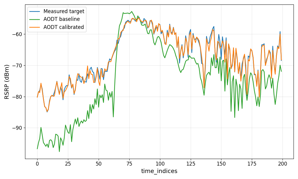
5.1 Reproducing the predicted-vs-measured curve overlap

The calibration comparison curve in §3.5 Training overlays the measured power against the predicted power along the UE route. It is produced in this post-processing stage by running the post-calibration simulation with the calibration outputs applied, then comparing the result against the original field measurements; a good calibration makes the two curves overlap.

How post-processing works

At a high level the stage takes the calibration outputs and field measurements as input, then runs four steps — fetch the beamforming artifacts, run a simulation from the §4 Calibrated simulation configuration, apply beamforming to the simulation results, and plot the predicted power against the measurements:

The rest of this section details the input and each step.

Input

Everything the stage starts from lives in the calibration output location (S3/MinIO):

the beam codebook RU_*_codebook.csv — the per-RU beam weights, present only when beam training was enabled (shown below);
the measurement traces — one RSRP (Reference Signal Received Power) CSV per RU–UE link, plus the optional per-link beam CSVs when beams are involved;
the §4 Calibrated simulation configuration sim_config_calibrated.yml — points a follow-up simulation at the recovered materials, vegetation, UE trajectory, RU orientation, and panels.

Running that follow-up simulation (step 2 below) produces the channel data (Iceberg/Parquet) carrying the CFR (Channel Frequency Response) that beamforming (step 3) consumes.

The codebook is the same artifact described in §4 RU beams output:

RU_1_codebook.csv

1 HorizontalElements 4
2 VerticalElements 4
3 DualPolarized 0
4 HorizontalSpacing 0.5
5 VerticalSpacing 0.5
6 Frequency_Hz 3619000000.0
7 Beam_idx, Tilt_deg, Azimuth_deg, Ant_re_0, Ant_im_0, ... , Ant_re_15, Ant_im_15
8 0, 100.000000, 0.000000, 0.683465, -0.729984, ... , 0.683465, 0.729984
9 1, 106.000000, 0.000000, 0.268548, -0.963266, ... , 0.268548, 0.963266
10 2, 112.000000, 0.000000, -0.193272, -0.981145, ... , -0.193272, 0.981145

Workflow

Each step is a block with its own input and output.

1 · Fetching — pull the beamforming artifacts from their store.

After fetching, the output folder is organized like this:

beamforming_outputs/
├── sim_config_calibrated.yml      # §4 Calibrated simulation configuration
├── RU_1_codebook.csv              # beam codebook (only when beams were trained)
├── ru1_ue1_with_beams_filled.csv  # per-link measurement-beam CSVs
└── ru2_ue1_with_beams_filled.csv

2 · Run simulation — run the post-calibration simulation with §4 Calibrated simulation configuration, the fetched sim_config_calibrated.yml file. This is the simulation immediately after calibration, not the initial simulation from §2 Simulation setup. Point it at fresh output locations so it does not overwrite the baseline simulation database. This regenerates the channel data for the calibrated scene and produces the predicted power.

3 · Apply beamforming — beamform the channel data from step 2 using the fetched codebook from step 1. When no codebook exists (RUsBeams was not true), a single antenna element is used as a baseline.

The output beamformed_rsrp.json holds the predicted RSRP per RU → UE → beam, as a time array and the matching power values in dBm:

beamformed_rsrp.json

1 {
2   "RU_1": {
3     "UE_1": {
4       "BEAM_0": {
5         "time_array": [0, 1, 2, 3],
6         "rsrp_dbm": [-65.2, -64.8, -66.1, -65.5]
7       },
8       "BEAM_1": {
9         "time_array": [0, 1, 2, 3],
10         "rsrp_dbm": [-67.0, -66.4, -67.9, -67.2]
11       }
12     }
13   }
14 }

4 · Plotting — overlay the curves; the degree of overlap is the visual check on the calibration result.

Table of Contents

1. Introduction

Simple calibration file bundle

campaign/

sim.yml

cal.yml

gpx/route_10.gpx

measurements/ru1_ue1_rsrp.csv

measurements/ru2_ue1_rsrp.csv

2. Simulation setup

2.1 UEs

Configuration snippet

Using existing campaign data

Limitations

2.2 RUs

Configuration snippet

Using existing campaign data

Limitations

2.3 Scenario

Configuration snippet

Limitations

2.4 DU frequency settings

Configuration snippet

Using existing campaign data

Limitations

2.5 Unsupported or ignored settings

3. Calibration

3.1 Importing from the previous simulation

3.2 Power measurements

3.3 Calibration targets

Materials

Vegetation Materials

UE calibration target

RU calibration target

RU beams calibration target

3.4 Defining the calibration run

Timeline — time-step selection

Measurements — per-link inputs

3.5 Training

Understanding the loss

Limitations

4. Outputs

Output folder tree

cal.output.folder_key

Calibrated/

Assets/

Materials/

Vegetation/

UEs_gpx/

Codebooks/

Calibrated building-material outputs

materials_calibrated.json + association.json

Vegetation material outputs

veg_materials_calibrated.json + association.json

Calibrated RU outputs

Calibrated UE outputs

ue_1_trajectory.gpx

Calibrated RU beam outputs

RU_1_codebook.csv

Calibrated simulation configuration

sim_config_calibrated.yml

5. Post-processing

5.1 Reproducing the predicted-vs-measured curve overlap

How post-processing works

Input

RU_1_codebook.csv

Workflow

beamformed_rsrp.json