

UI
The AODT viewer is a CesiumJS-based web application for working with simulation scenarios on a 3D geospatial map. It renders city-scale 3D Tiles and quantized mesh terrain from S3, displays radio access network (RAN) entities, and visualizes ray-traced signal paths colored by received power. The viewer can load simulation YAML, edit scenario entities, connect to an Iceberg catalog, and play back time-indexed simulation data.
For installation steps, see Viewer Installation.
Prerequisites
Before using the viewer, confirm:
- The viewer is installed and running.
- Scene assets are available in S3 under a
gis.scene.scene_urlpath. - A simulation YAML file or database connection settings are available.
- Raypath data has been exported to Iceberg/Parquet if signal visualization is needed.
Viewer Workflow
A typical viewer workflow:
- Load a simulation YAML file with Upload YML. The viewer automatically applies the configuration — 3D Tiles and terrain load from the scene path, entities (RUs, DUs, UEs, panels, spawn zone) appear on the map, and database connection fields are populated from the YAML.
- Verify that the scene and entities appear as expected.
- Create, move, rotate, or edit entities from the viewport and right sidebar.
- Download the updated YAML from the editor and use it to run a simulation with the AODT Client.
- Visualize simulation results by connecting to a database in Settings.
Layout
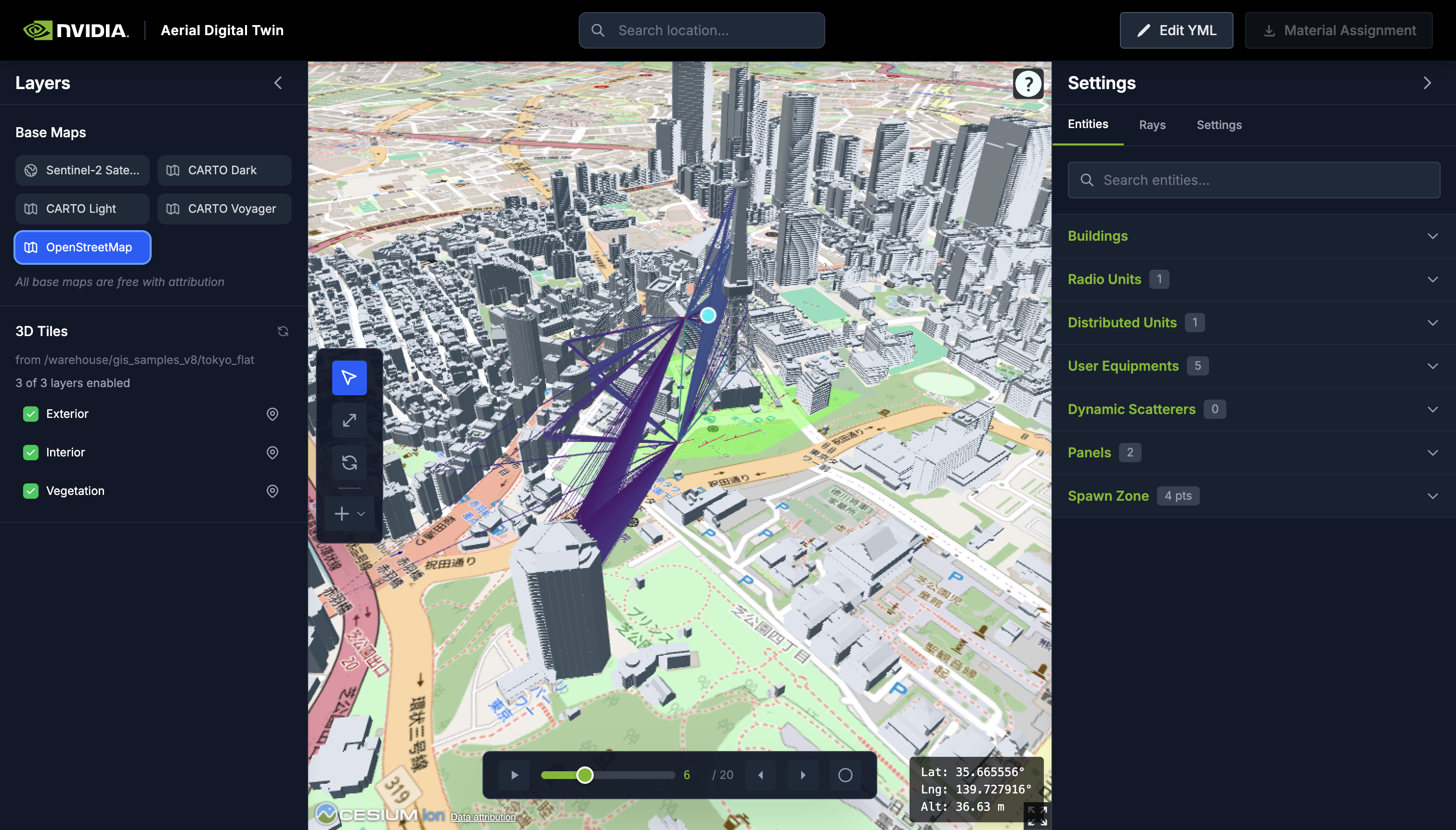
The viewer is a single-screen application with five regions:
- Top header — location search, YAML editor access, and material assignment export.
- Left sidebar — base map selection and 3D Tiles layer controls.
- 3D viewport — the CesiumJS globe where entities, buildings, terrain, and raypaths are rendered.
- Right sidebar — Entities for entity lists and property editors, Rays for signal visualization controls, and Settings for database connection and map options.
- Timeline — bottom bar for stepping through simulation time indices.
Layers
The left sidebar controls the map layers:
- Base Maps — OpenStreetMap (default), CARTO Dark/Light/Voyager, Sentinel-2, or Cesium Ion Satellite. Cesium Ion Satellite requires an Ion token in Settings.
- Terrain — high-detail quantized-mesh terrain loaded from the scene’s S3 path when the camera is below about 50 km altitude. At higher altitudes the viewer switches to an ellipsoid for performance.
- 3D Tiles — building exteriors, interiors, and vegetation loaded from the
viz/tiles/path derived fromgis.scene.scene_url. Each layer can be toggled independently.
Click any building to view its properties (name, surface hash, material) in the right sidebar. Hover highlights buildings with a blue silhouette; selection highlights in green.
Entities
The viewer supports editing and visualizing five entity types and a spawn zone. All except scatterers can be created directly in the UI. Each entity in the sidebar has a magnifying glass icon that focuses the camera on that entity when clicked.
Editing tools
The toolbar on the left edge of the viewport provides four tools:
- Select — click to pick buildings or entities.
- Move — drag an entity to reposition it.
- Rotate — adjust an RU’s azimuth and tilt.
- Create — place a new RU, DU, UE, panel, or spawn zone.
Entity changes sync back into the stored YAML automatically. See Configuring Sim YAML in the UI for details.
Radio Unit (RU)
Click Create → Radio Unit, then click a location on the map. The RU projects onto both terrain and building surfaces, so it can be placed on rooftops or walls. A red 3D model with a label appears at the placed position.
In the sidebar you can edit: cell ID, DU assignment (automatic or manual), panel type, radiated power (-20 to 80 dBm), height (0.5 to 100 m), mechanical azimuth and tilt (0 to 360°), and a per-RU rays toggle. When DU assignment is set to automatic, the viewer assigns the closest DU whose panel type matches.
Use the Rotate tool (RU only) to adjust azimuth and tilt with ring gizmos directly on the map.
Distributed Unit (DU)
Click Create → Distributed Unit, then click a location. Like RUs, DUs project onto both terrain and building surfaces on placement.
Editable properties: subcarrier spacing (15 to 960 kHz), FFT size (256 to 4096), reference frequency, and number of antennas (1 to 64). Max channel bandwidth is displayed but read-only.
User Equipment (UE)
Click Create → User Equipment, then click a location. UEs snap to terrain rather than buildings. The viewer creates a manual UE with one initial waypoint at the clicked position.
Editable properties: panel type, radiated power, mechanical tilt, and height (0 to 10 m). The type (manual or procedural), mobility mode, and environment (indoor/outdoor) are shown but not editable. Procedural UEs loaded from a database have no editable waypoints.
Waypoints
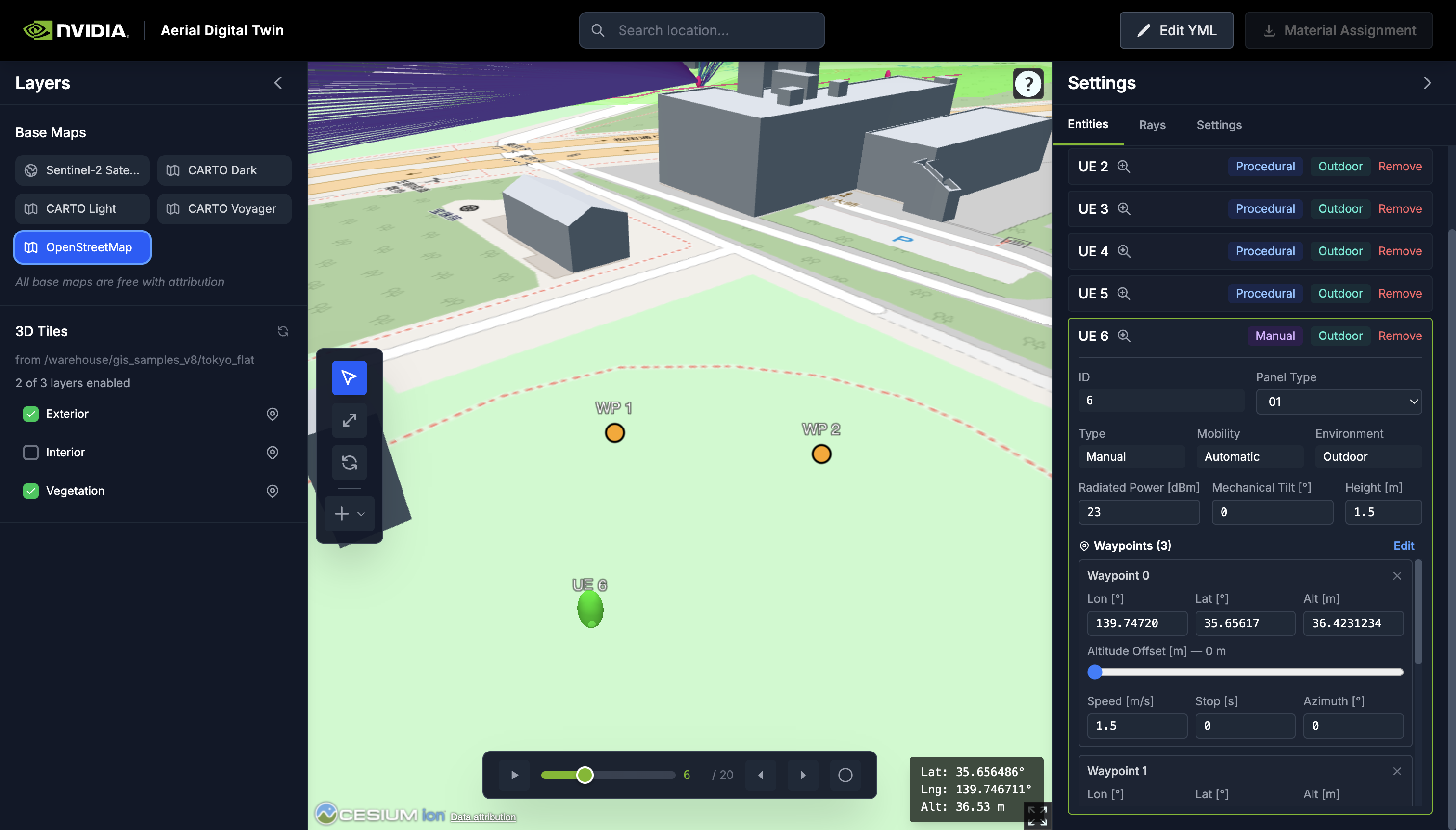
To define a movement path, expand the UE in the sidebar and click Edit on the waypoints section. This enters waypoint placement mode — click terrain to add points. Each waypoint has editable speed, stop time, azimuth, and an altitude offset (0 to 500 m). Click Done to commit or Cancel to discard. Only one UE can edit waypoints at a time.
Manual UEs created in the viewer default to 2D mobility — the UE and its waypoints are projected onto the terrain surface. Setting any waypoint’s altitude offset to a non-zero value switches that UE to 3D mobility. When using 3D mobility, make sure the UE and all of its waypoints are clear of buildings and terrain to avoid collision failures during pathfinding.
Panel
Click Create → Panel. Panels have no map representation — creation immediately adds the panel to the sidebar. A grid visualizer shows the antenna layout.
Editable properties: polarization (single or dual), horizontal and vertical antenna count, antenna spacing (cm), roll angles for each polarization, reference frequency, and antenna type.
Spawn Zone
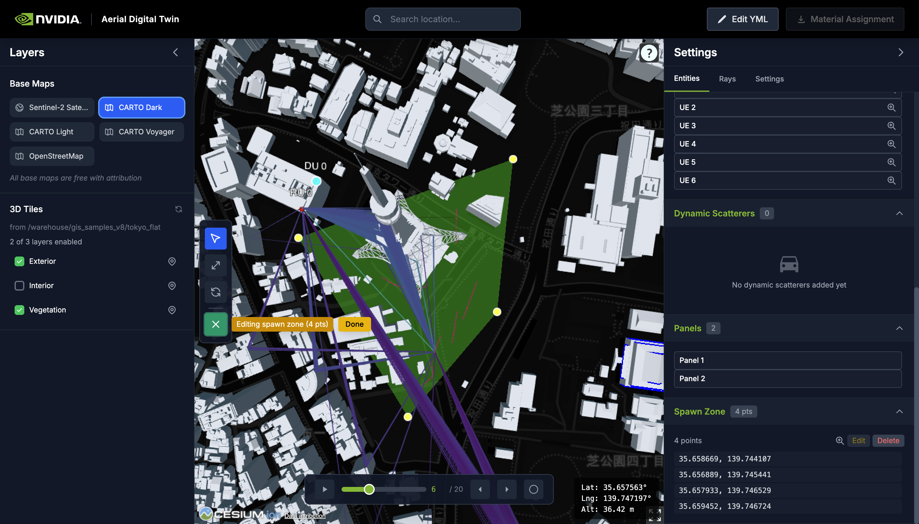
Click Create → Spawn Zone, then click terrain to place polygon vertices. Spawn zone points project onto the ground only, not buildings. After three or more points, the viewer computes and displays the convex hull as a green polygon that follows the terrain surface. Only the convex hull is visualized — if points are placed in a concave arrangement, the displayed polygon will be their convex hull. Click an existing point to remove it, or drag points to reposition them. Click Done to commit.
The spawn zone section in the sidebar shows the point coordinates and provides Edit (re-enter point mode), Delete (clear), and zoom controls. Creating a new spawn zone replaces any existing one.
Scatterers
Scatterers cannot be created in the viewer. They are loaded from a database as time-indexed positions and orientations, typically representing vehicles. Properties (ID, environment) are read-only. The Move tool can reposition a scatterer at the current time index, but routes and other properties cannot be edited.
Rays
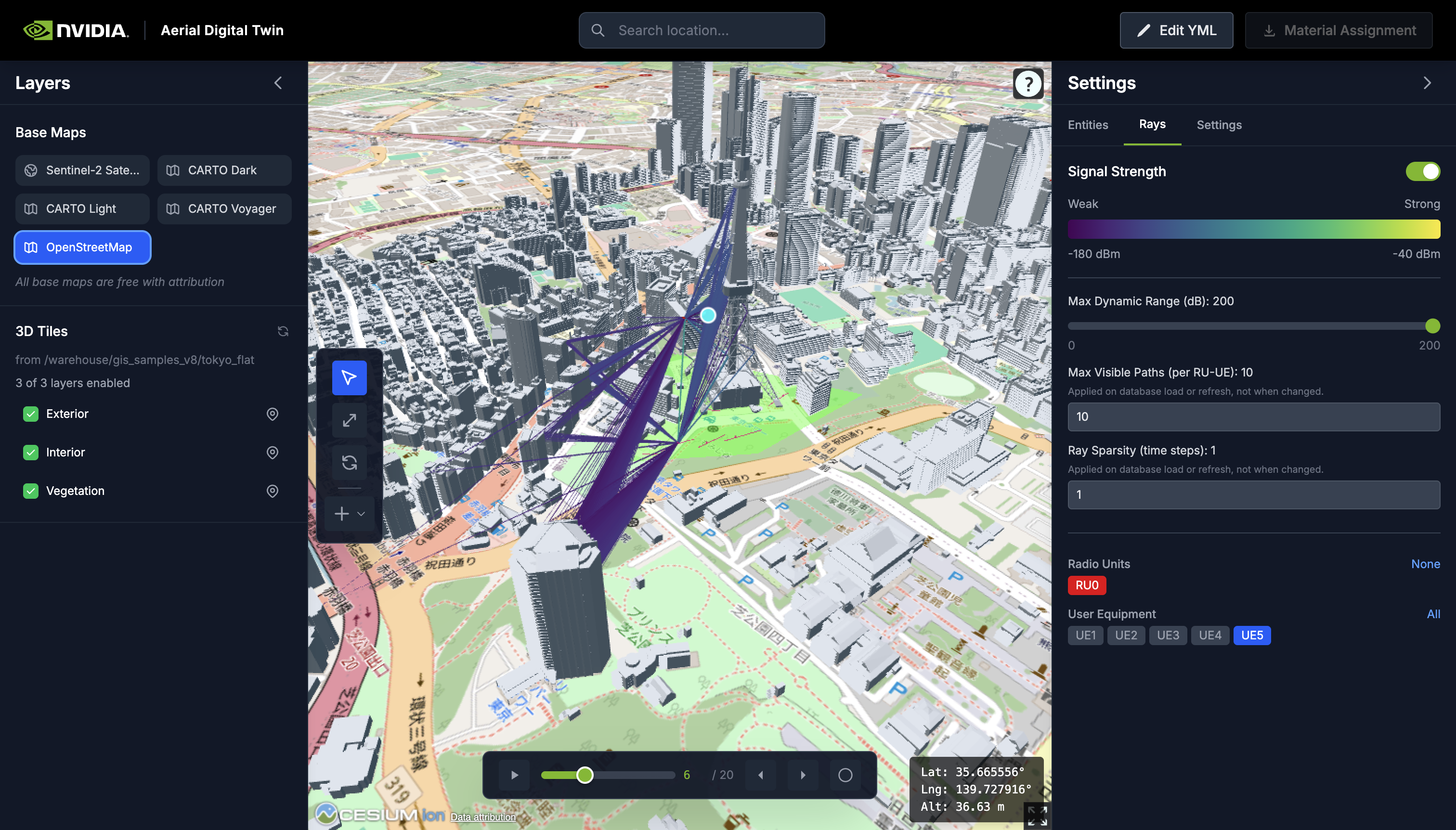
After loading simulation results from a database, the viewer renders ray-traced signal paths as 3D polylines colored by received power (-180 to -40 dBm).
The Rays tab in the right sidebar provides:
- Visibility toggle — show or hide all raypaths.
- Max dynamic range — a slider from 0 to 200 dB that hides paths below
max(power) - range. This updates in real time. - Max visible paths and ray sparsity — cap the number of loaded paths per RU-UE pair and subsample time steps. These settings apply on the next database load or refresh.
- RU/UE filters — toggle individual RUs and UEs.
See Telemetry for interpretation guidance.
Timeline
The timeline bar at the bottom appears after connecting to a database or uploading a YAML with simulation parameters.
- Play / Pause — step through time indices automatically at a configurable interval.
- Scrubber — drag to jump to any time index.
- Go to — type a specific time index.
- Step — advance or go back one index at a time.
The current time index drives entity visibility: UE and scatterer positions update to match the selected time step, and raypaths are filtered to show only paths computed at that index. Mobility traces from all batches are displayed simultaneously to show the spatial coverage of mobility generation across batches.
Settings
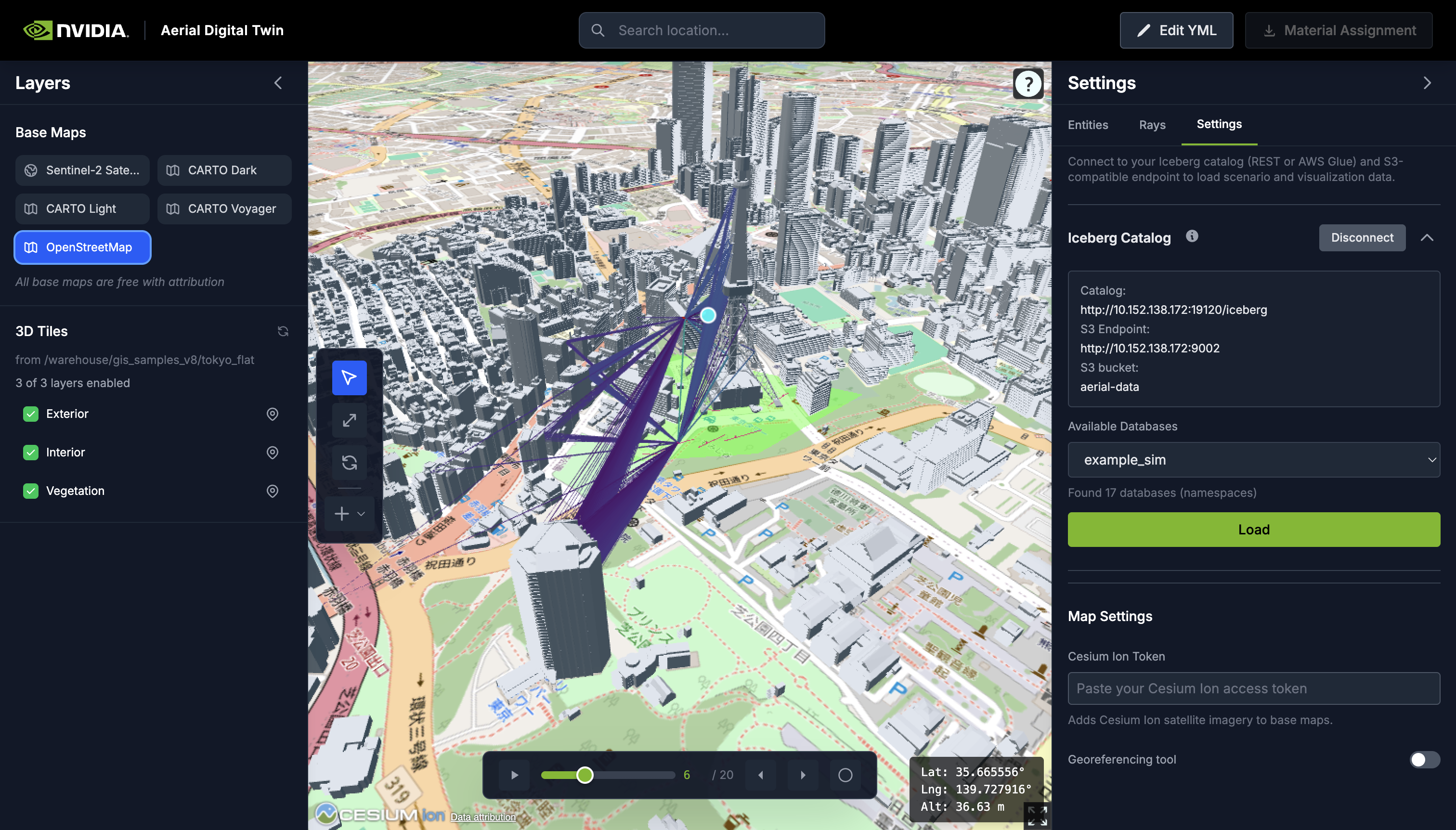
Open the Settings tab in the right sidebar to connect to simulation data:
- Choose a catalog type: REST (e.g. Nessie) or AWS Glue.
- Enter the catalog URI or AWS region.
- Set the S3 provider (MinIO or AWS), endpoint, bucket, and optional credentials.
- Click Connect, select a database namespace, then Load.
The viewer fetches entity positions, scenario parameters, panel configurations, and raypaths from Iceberg/Parquet tables in S3. Loading from the database overrides any entities and parameters from the current YAML. Use Refresh to reload after a new simulation run.
These connection fields can also be populated from the db section of an
uploaded YAML file.
Related Pages
Raypath interpretation and time-indexed signal analysis.
Upload, edit, and export simulation YAML from the viewer.
- See Viewer Installation for prerequisites and setup.
- See Scene Generation for how 3D Tiles and terrain are built from geospatial data.
- See Configuring Sim YAML for the programmatic YAML workflow and Config Builder.