Introduction to EM Physics

1. Introduction

The EM engine predicts how a radio-frequency (RF) field radiated by a transmit antenna propagates through a geometric environment — buildings, terrain, vehicles, vegetation — and arrives at one or more receivers. The output is a set of propagation paths, each carrying a complex (amplitude + phase) vector field, from which we derive channel impulse responses (CIRs) and channel frequency responses (CFRs), angles of departure, angles of arrival, delays, and MIMO channel matrices for downstream applications (e.g. RAN system simulations).

Solving Maxwell’s equations directly in a scene that is hundreds or thousands of wavelengths across (a ~100 m city block at 3 GHz spans ~ $10^3\,\lambda$ ) by full-wave methods (finite-difference time-domain (FDTD), method of moments (MoM), finite element method (FEM)) is computationally impractical for large-scale system-level work. Instead we exploit the fact that at high frequency the wavelength is tiny compared with the scene features, so energy travels along well-defined trajectories that behave locally like rays of light. This is the domain of Geometrical Optics (GO) and its diffraction-aware extension, the Uniform Theory of Diffraction (UTD). The EM engine’s RF ray-tracer is the tool that models this physics: it finds the ray-path trajectories, and applies the EM field calculation along each trajectory taking into account the antenna emission and reception fields.

2. Finding Propagation Paths by Ray Tracing

Before any EM is applied, the engine finds the valid ray-path trajectories connecting each of the transmit antennas to each of the receive antennas. The trajectories must obey the relevant optical laws (Snell’s law of reflection, Keller’s law of diffraction, or straight-through propagation for transmission) and must not be blocked by any geometry.

2.1 Finding ray paths with NVIDIA OptiX

For large and complex scenes with a high level of geometric detail, the ray paths are efficiently found by ray tracing using the Shooting and Bouncing Rays (SBR) technique. A dense bundle of initial rays is launched from each transmitter over the sphere of directions; each ray is propagated and intersected with the geometry, and depending on the EM interaction type at the intersection, the ray either changes direction (specular reflection or transmission through the interface) or spawns secondary rays (for diffraction and diffuse scattering). The ray tracing module uses NVIDIA OptiX [1] and runs on modern GPU ray-tracing hardware (RT cores traversing a bounding volume hierarchy) to accelerate the path finding.

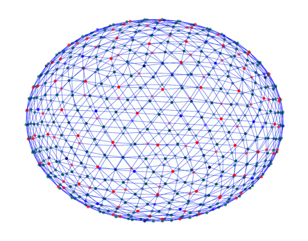
To sample the launch directions of the initial rays, the engine uses sphere points on icosahedral grids [2], which have good distributions — that is, near-uniform nearest-neighbor spacing and angular density.

Because a shot ray almost never passes exactly through the receiver point, a reception sphere is placed at each of the receive points to capture the preliminary candidate ray paths. This is followed by a path refinement step, so that the final ray paths pass through the receive points exactly and satisfy the relevant optical laws, using the previously stored interaction sequence and intersecting geometries. Identical paths for a given Tx–Rx antenna pair — those sharing the same interaction sequence and intersecting geometries — are then deduplicated.

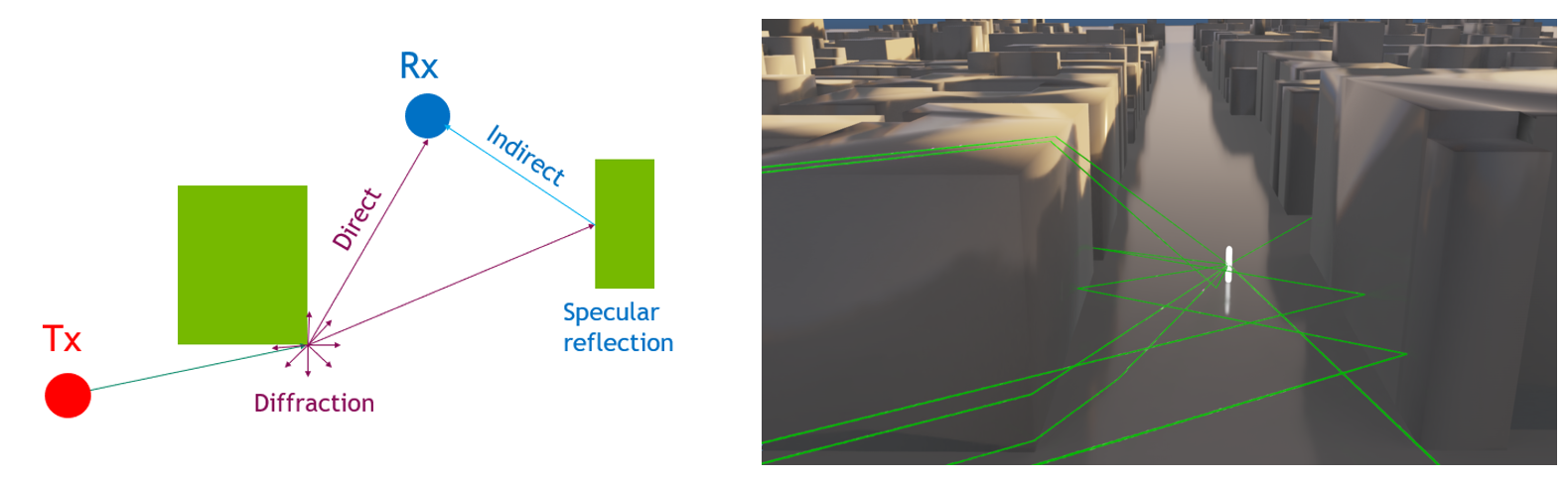
A ray-path trajectory from an emission point (Tx) to a reception point (Rx) may not interact with any geometry (a line-of-sight path), may pass through multiple specular reflection bounces, or may combine diffraction and reflection bounces.

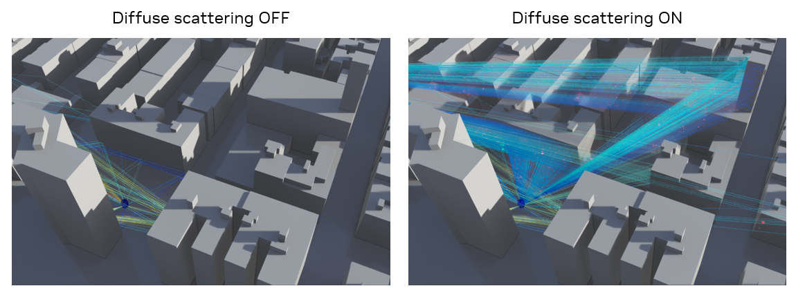
When diffuse scattering is enabled at an interaction (with buildings, cars, or vegetation), the interacting surface is discretized into small surface elements, and secondary rays are spawned diffusely from each element. Each diffuse ray carries a fraction of the element’s total diffused power, scaled proportionally to the surface element’s area.

2.2 Higher-order interactions and path data pruning

A path’s interaction order (the number of interaction events between the Tx and Rx) is capped at a maximum (MAX_NUM_INTERACTIONS), so a traced ray is terminated once it is missed or its number of interactions exceeds this cap. Furthermore, the engine lets the user set a maximum number of strongest (by power) ray paths to retain for each Tx/Rx antenna pair.

3. EM Field Modeling

The EM calculation walks each path from Tx to Rx, starting with the radiated field, applying one field transfer matrix per bounce to transport the field along each segment, and finally projecting onto the receive antenna. The field is always a transverse complex vector, tracked in a ray-fixed coordinate system ( $\vec{r},\; \vec{\theta},\; \vec{\phi}$ ) so that ( $\theta$ / $\phi$ or vertical/horizontal) polarizations are handled correctly.

3.1 Emission from the transmit antenna

The electric field radiated by a transmit antenna is modeled using its gain $G_{\text{Tx}}$ and its far-field radiation patterns, described in vector form as $\begin{bmatrix} E_{\theta}^{\text{Tx}}\left(\theta^{\text{Tx}}, \phi^{\text{Tx}}\right) \\ E_{\phi}^{\text{Tx}}\left(\theta^{\text{Tx}}, \phi^{\text{Tx}}\right) \end{bmatrix}$ at angle $\left(\theta^{\text{Tx}}, \phi^{\text{Tx}}\right)$ in the spherical coordinate system. At the far-field distance $r_0$ , the radiated field by the emission in the free-space is expressed as

\begin{bmatrix} \vec{E}_\theta^\text{Tx}\left(r\right) \\ \vec{E}_\phi^\text{Tx}\left(r\right) \end{bmatrix} = \left(E_0\sqrt{G_\text{Tx}}\right) \begin{bmatrix} E_{\theta}^{\text{Tx}}\left(\theta^{\text{Tx}}, \phi^{\text{Tx}}\right)\vec{\theta}^{\text{Tx}} \\ E_{\phi}^{\text{Tx}}\left(\theta^{\text{Tx}}, \phi^{\text{Tx}}\right)\vec{\phi}^{\text{Tx}} \end{bmatrix} \frac{1}{r_0}e^{-jkr_0}

where $E_0 = \sqrt{\frac{P_tZ_0}{2\pi}}$ is the relative amplitude of the spherical source, $k = \frac{2\pi}{\lambda}$ is the wave number, and $\lambda$ is the wavelength.

3.2 Field transfer along the EM interactions

For each path containing $I$ EM interactions, denote the field transfer matrix by the interaction (reflection, transmission, diffraction, diffusion) $i\ (i = 1, 2,...,\ I)$ as $F_i = \begin{bmatrix} F_{\theta\theta}^i & F_{\phi\theta}^i \\ F_{\theta\phi}^i & F_{\phi\phi}^i \end{bmatrix}$ , where $F_{xy}^i$ is the field transfer coefficient for receive polarization $x$ and transmit polarization $y$ , where $x, y \in \{\theta, \phi\}$ . Denote $S_i$ as the spreading factor on the following segment $r_i$ after the $i$ -th interaction. The composite effect on the field for each path when it propagates from the Tx, going through interactions with the environment, reaching the Rx antenna can be expressed as

\left(\prod_{i=I}^0F_iS_i\right)e^{-jk\sum_{i=0}^Ir_i}

where $F_0 = \begin{bmatrix} 1 & 0 \\ 0 & 1 \end{bmatrix}$ and the spreading factor $S_0 = \frac{1}{r_0}$ for the emission from the spherical source are included.

In what follows, the $F_i$ and $S_i$ for each EM interaction type are described.

3.2.1 Fresnel reflection and transmission

When a ray meets a locally planar interface between free space and a material with complex relative permittivity

\varepsilon_r = \varepsilon_r' - j\,\frac{\sigma}{\omega\varepsilon_0} = \varepsilon_r' - j\,60\,\lambda\,\sigma,

(with $\sigma$ the conductivity in S/m and $\lambda$ in meters; the $60\lambda\sigma$ form follows from $\sigma/(\omega\varepsilon_0)=\sigma\lambda/(2\pi c\varepsilon_0)\approx 60\lambda\sigma$ ), the field splits into two independent polarizations defined relative to the plane of incidence (the plane containing the incident ray and the surface normal):

Perpendicular/TE ( $\perp$ ): the field is perpendicular to the plane of incidence;
Parallel/TM ( $\parallel$ ): the field is in the plane of incidence.

With incidence angle $\theta_i$ from the normal and $\mu_r=1$ , the Fresnel reflection coefficients are

R_\perp = \frac{\cos\theta_i - \sqrt{\varepsilon_r - \sin^2\theta_i}}{\cos\theta_i + \sqrt{\varepsilon_r - \sin^2\theta_i}}, \qquad R_\parallel = \frac{\varepsilon_r\cos\theta_i - \sqrt{\varepsilon_r - \sin^2\theta_i}}{\varepsilon_r\cos\theta_i + \sqrt{\varepsilon_r - \sin^2\theta_i}},

and the transmission (refraction) coefficients for the field crossing into the material are

T_\perp = \frac{2\cos\theta_i}{\cos\theta_i + \sqrt{\varepsilon_r - \sin^2\theta_i}} = 1 + R_\perp, \qquad T_\parallel = \frac{2\sqrt{\varepsilon_r}\,\cos\theta_i}{\varepsilon_r\cos\theta_i + \sqrt{\varepsilon_r - \sin^2\theta_i}}.

By Snell’s law, the reflected ray leaves at $\theta_r = \theta_i$ , on the far side of the normal. The transmitted ray bends at the angle $\theta_t$ such that $\sin\theta_t = \sin\theta_i/\sqrt{\varepsilon_r}$ (complex for lossy media).

The field transfer matrix for the reflection is

\mathbf{F}_i^{(\text{R})} = \mathbf{M}_o^{(\text{R})} \begin{bmatrix} R_\perp & 0 \\ 0 & R_\parallel \end{bmatrix} \mathbf{M}_i^{(\text{R})}

where $\mathbf{M}_i^{(\text{R})}$ is the matrix transforming the ray-fixed coordinates to the incident-plane aligned coordinates $\left(\vec{k}_i,\;\vec{e}_{\perp},\;\vec{e}_{\parallel,i}\right)$ of the incident electric field (in the direction $\vec{k}_i$ ), $\mathbf{M}_o^{(\text{R})}$ is the matrix transforming the incident-plane aligned coordinates $\left(\vec{k}_r,\;\vec{e}_{\perp},\;\vec{e}_{\parallel,r}\right)$ back to the ray-fixed coordinates of the outgoing electric field (in the direction $\vec{k}_r$ ). Since in general, $\mathbf{M}_{i/o}^{(\text{R})}$ is not the unity matrix, an incident field in one polarization results in fields in both outgoing polarizations — this is the physical origin of the cross-polarization of the EM propagation interactions.

Similarly, the field transfer matrix for the transmission is

\mathbf{F}_i^{(\text{T})} = \mathbf{M}_o^{(\text{T})} \begin{bmatrix} T_\perp & 0 \\ 0 & T_\parallel \end{bmatrix} \mathbf{M}_i^{(\text{T})},

where $\mathbf{M}_i^{(\text{T})} = \mathbf{M}_i^{(\text{R})}$ , and $\mathbf{M}_o^{(\text{T})}$ is the matrix transforming the incident-plane aligned coordinates $\left(\vec{k}_t,\;\vec{e}_{\perp},\;\vec{e}_{\parallel,t}\right)$ back to the ray-fixed coordinates of the outgoing electric field (in the direction $\vec{k}_t$ ). For the transmission through a thin single-layer slab, the direction of the outgoing ray is assumed to remain unchanged.

Finite walls (slabs). The coefficients above are for a semi-infinite half-space. For a wall of finite thickness $d$ , the engine can instead use a single-layer slab reflection/transmission model [3], $R_{\perp/\parallel,\ \text{slab}} = R_{\perp/\parallel}\frac{1-e^{-2jq}}{1 - R_{\perp/\parallel}^2e^{-2jq}}, \qquad T_{\perp/\parallel,\ \text{slab}} = \frac{(1-R_{\perp/\parallel}^2)\,e^{-jq}}{1 - R_{\perp/\parallel}^2 e^{-2jq}}$ where $q = kd\sqrt{\varepsilon_r - \sin^2\theta_i}$ . The model produces the frequency-dependent ripple and extra reflection and transmission loss that more realistic walls exhibit.

The spreading factor on the following segment after the reflection/transmission $i$ is

S_i^{\text{(R/T)}} = \frac{\rho}{\rho + r_i},

where $\rho = \sum_{k=0}^{i-1}r_k$ is the radius of curvature of the spherical wave impinging on the surface at the $i$ -th interaction, and $r_i$ is the length of the following segment.

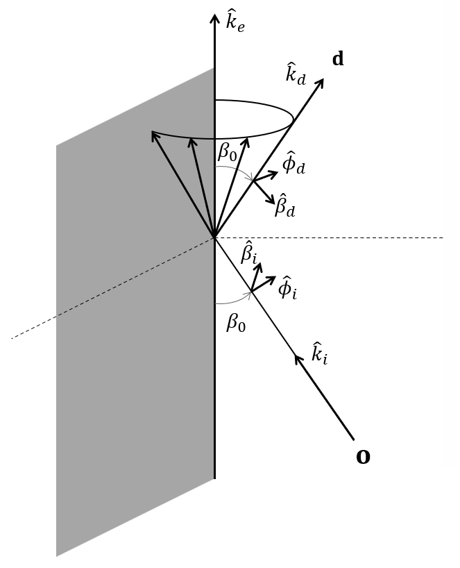
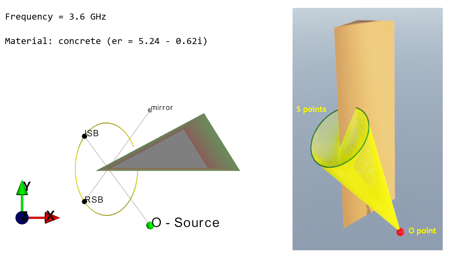
3.2.2 Diffraction — the UTD wedge

When a ray strikes an edge (the intersection of two planar faces forming a wedge of exterior angle $n\pi$ ), it launches a Keller cone of diffracted rays: all diffracted rays make the same angle $\beta_0$ with the edge as the incident ray does (the “law of edge diffraction”), so they form a cone about the edge. The diffracted field transfer matrix is expressed as

\mathbf{F}_i^{(\text{D})} = \mathbf{M}_o^{(\text{D})} \mathbf{D} \mathbf{M}_i^{(\text{D})},

where $\mathbf{D}$ is the $2\times2$ matrix containing four diffraction coefficient terms [4], $\mathbf{M}_i^{(\text{D})}$ is the matrix transforming the ray-fixed coordinates to the edge-fixed coordinates $\left(\vec{k}_i,\;\vec{\beta}_i,\;\vec{\phi}_i\right)$ of the incident electric field (in the direction $\vec{k}_i$ ), $\mathbf{M}_o^{(\text{D})}$ is the matrix transforming the edge-fixed coordinates $\left(\vec{k}_d,\;\vec{\phi}_d,\;\vec{\beta}_d\right)$ back to the ray-fixed coordinates of the outgoing electric field (in the direction $\vec{k}_d$ ).

The diffraction coefficient matrix is calculated as

\begin{aligned} \mathbf{D} =& -D^-(\phi_d - \phi_i)\mathbf{\Omega_0} -D^+(\phi_d - \phi_i)\mathbf{\Omega_n} \\ & + D^-(\phi_d + \phi_i)\mathbf{M_0^{''}}\mathbf{R_0(\alpha_0)}\mathbf{M_0^{'}} \\ & + D^+(\phi_d + \phi_i)\mathbf{M_n^{''}}\mathbf{R_n(\alpha_n)}\mathbf{M_n^{'}}; \end{aligned}

where

D^{\mp}(x) = \frac{-e^{-j(\pi/4)}}{2n\sqrt{2\pi k}\sin \beta_i}\text{cot}\left(\frac{\pi \mp x}{2\pi}\right)F\left[kLa^{\mp}(x)\right],

a^\mp(x) = 2\cos^2\left(\frac{2n\pi N^\mp - x}{2}\right),

with $N$ being the closest integers for which the following relationships are satisfied

2\pi nN^{\mp} - x = \mp \pi.

The transition function $F$ is defined as

F(x) = 2j\sqrt{x}e^{jx}\int_{\sqrt{x}}^{\infty}e^{-j\tau^2}d\tau,

$\mathbf{R_{0/n}(\alpha_{0/n})} = \begin{bmatrix} R_\perp(\alpha_{0/n}) & 0 \\ 0 & R_\parallel(\alpha_{0/n}) \end{bmatrix}$ is the reflection coefficient matrix for face $0/n$ with incidence angle $\alpha_{0/n}$ . $\mathbf{M_{0/n}^{'}}$ is the rotation matrix transforming the edge-fixed coordinates to the incident-plane aligned coordinates considering incident ray at face-0/n. $\mathbf{M_{0/n}^{''}}$ is the rotation matrix transforming the incident-plane aligned coordinates back to the edge-fixed coordinates considering incident ray at face-0/n.

The angles $\alpha_0$ and $\alpha_n$ are functions of $\phi_i$ and $\phi_d$ , depending on whether face-0, face-n, or both are illuminated, following the formulation in [5] to achieve the reciprocity of the diffraction coefficients.

The spreading factor on the following segment after the diffraction $i$ is

S_i^{(\text{D})} = \sqrt{\frac{\rho}{(\rho + r_i)r_i}},

where $\rho = \sum_{k=0}^{i-1}r_k$ is the radius of curvature of the spherical wave impinging on the surface at the $i$ -th interaction, and $r_i$ is the length of the following segment.

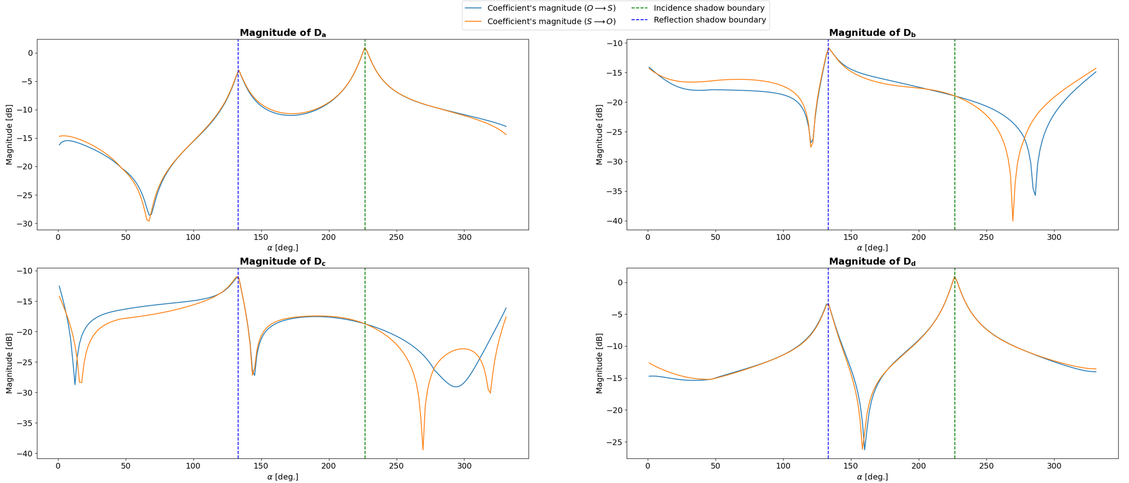
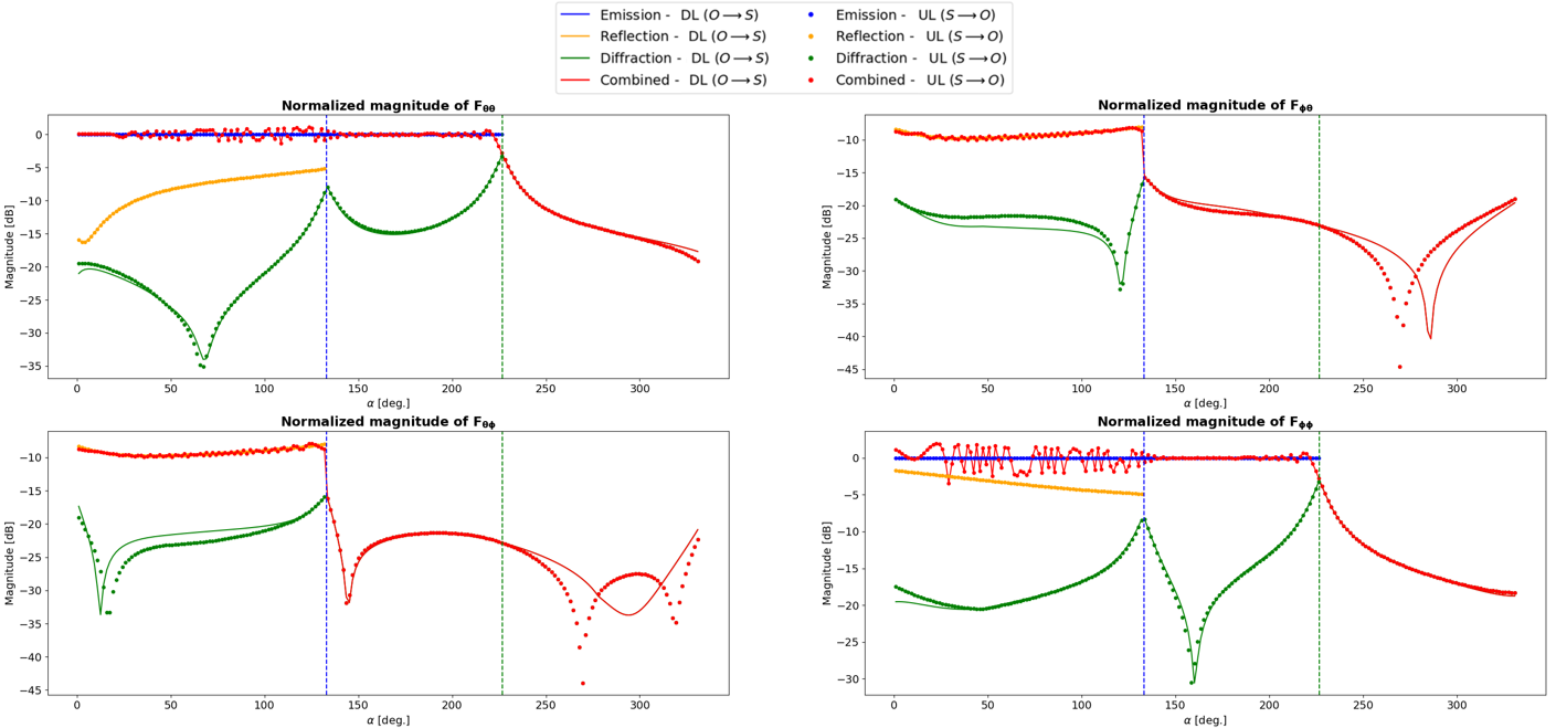
The following figures show the reciprocity of the model by comparing all four diffraction coefficients, as well as the combined ones, generated by the EM engine for a triangular prism setup for both incident directions: (i) O $\rightarrow$ S: O is Tx, S is Rx, and (ii) S $\rightarrow$ O: S is the Tx, O is the Rx.

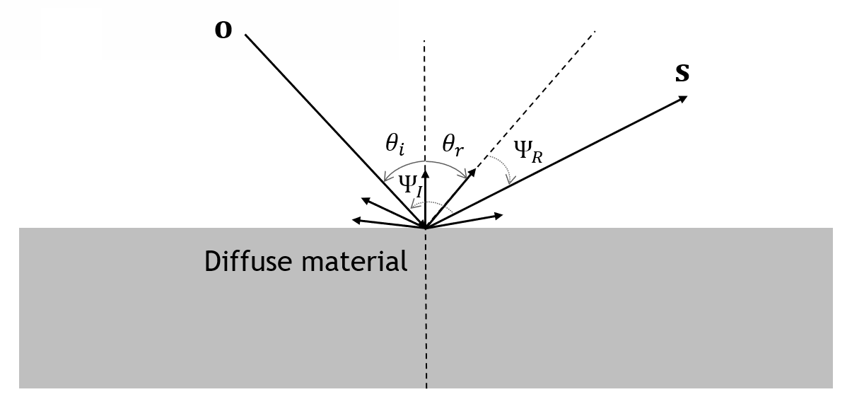
3.2.3 Surface diffuse scattering

GO/UTD assume smooth surfaces — they put all the reflected energy into the single specular direction. Real surfaces (brick, rough concrete) are rough on the wavelength scale and scatter energy diffusely into a broad lobe. The engine supports two surface diffuse scattering models: the Lambertian model and the more directional model [6], which is an extension of the effective roughness (ER) model [7]. Both supported models are reciprocal.

The field transfer matrix for the surface scattering interaction is expressed as

\mathbf{F}_i^{(S)} = \mathbf{M}_o^{(S)} \begin{bmatrix} S_\text{scat}\sqrt{\dfrac{1}{1+k_x}}R_\perp\tilde{S} & S_\text{scat}\sqrt{\dfrac{k_x}{1+k_x}}R_\parallel\tilde{S} \\ S_\text{scat}\sqrt{\dfrac{k_x}{1+k_x}}R_\perp\tilde{S} & S_\text{scat}\sqrt{\dfrac{1}{1+k_x}}R_\parallel\tilde{S} \end{bmatrix} \mathbf{M}_i^{(S)},

where $k_x$ is the cross-polarization ratio term, and $S_\text{scat}$ is the scattering coefficient. When using the root mean square (RMS) roughness to characterize the Rayleigh reflectance coefficient of the material [8], [9], $\rho_R = \exp\left[-\frac{1}{2}\left(4\pi\delta\cos\theta_i/\lambda\right)^2\right]$ , then $S_\text{scat} = \sqrt{1-\rho_R^2}$ . $\mathbf{M}_{i/o}^{(\text{S})}$ is the matrix to transform between the ray-fixed coordinates and the incident-plane aligned coordinates, similarly defined as in $\mathbf{M}_{i/o}^{(\text{R})}$ for the reflection interaction above.

Using Lambertian scattering model,

\tilde{S} = \sqrt{\frac{1}{\pi}\Delta S\cos\theta_i\cos\theta_d},

where $\Delta S$ is the area of the diffuse surface element, $\theta_i$ and $\theta_d$ are the angle of the incident ray and angle of the diffused ray (measured from the surface normal), respectively.

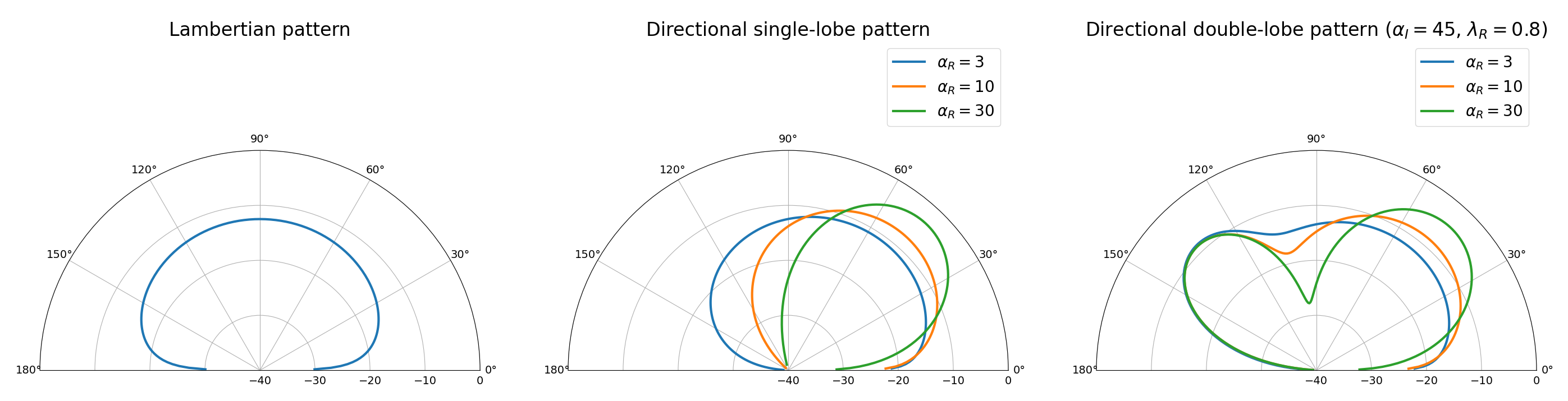
Using the directional/extended ER model, for the generic double-lobe model,

\tilde{S} = \sqrt{\frac{\Delta S\sqrt{\cos\theta_i\cos\theta_d}}{4\pi}\left[\Lambda_R\,F_{\alpha_R}\left(\frac{1 + \cos\Psi_R}{2}\right)^{\alpha_R} + (1-\Lambda_R)\,F_{\alpha_I}\left(\frac{1 + \cos\Psi_I}{2}\right)^{\alpha_I}\right]},

where

F_{\alpha} = \frac{2^{\alpha}}{\displaystyle\sum_{j=0}^{\alpha}\binom{\alpha}{j}\frac{1}{2j+3}},

and $\Psi_R$ is the angle between the diffused direction and the specular reflection direction, $\Psi_I$ is the angle between the diffused direction and the incident direction.

While the Lambertian model is governed by $S_\text{scat}$ only (either directly or via the roughness-dependent Rayleigh reflectance coefficient), the directional model is governed by $S_\text{scat}$ and the lobe-width exponent $\alpha_R$ for single-lobe directional model, or $(S_\text{scat},\;\alpha_R,\;\alpha_I,\;\Lambda_R)$ for the double-lobe directional model, where $\Lambda_R$ is the ratio between the forward scattering power and the total scattering power. When $\Lambda_R \to 1$ , $\tilde{S}$ becomes the single-lobe directional model. A larger $\alpha_R$ gives a narrower, more specular-like lobe. When $\alpha_R \to 0$ , the directional model becomes the Lambertian one. The following figure shows the diffuse scattering patterns for Lambertian (left), single-lobe directional (middle), and double-lobe directional (right) models with $S_\text{scat} = 0.25,\;\theta_i = 45^\circ$ .

Power conservation: With the presence of the surface diffuse scattering, the energy that goes into the diffusion must be removed from the coherent surface reflection, so the reflection coefficient is rescaled as

R_{\perp/\parallel} \; \longrightarrow\; \rho_RR_{\perp/\parallel}.

The rescaling also affects the diffraction coefficients using UTD approach above.

The spreading factor on the following segment $r_i$ after the diffuse scattering $i$ is

S_i^{(S)} = \frac{1}{r_i}.

3.2.4 Vegetation diffuse scattering

The engine supports diffuse scattering from vegetation, assuming an isotropic scattering pattern, i.e., same power in all directions over the unit sphere. The following figure illustrates the diffuse scattering (a) and transmission (b) modeling of vegetation interactions.

The attenuation loss is empirically modeled using ITU-R Recommendation P.833-10 [10] as:

L_\text{dB} = Af^{B}d^{C}(\theta + E)^{G},

where $f$ is the carrier frequency (in MHz), $d$ is the vegetation depth (in meters), $\theta$ is the path’s elevation angle (in degrees), and $A,\;B,\;C,\;E,\;G$ are the empirical model parameters. The coefficient matrix for the vegetation diffuse scattering is calculated as

\mathbf{S}^V = \begin{bmatrix} \sqrt{\dfrac{1}{1+k_x^V}}\,\tilde{S}^V & \sqrt{\dfrac{k_x^V}{1+k_x^V}}\,\tilde{S}^V \\ \sqrt{\dfrac{k_x^V}{1+k_x^V}}\,\tilde{S}^V & \sqrt{\dfrac{1}{1+k_x^V}}\,\tilde{S}^V \end{bmatrix}, \qquad \tilde{S}^V = \sqrt{\frac{1}{4\pi}S_\text{scat}^V(1 - 10^{-L_\text{dB}/10})\Delta S\cos\theta_i},

where $S_\text{scat}^V$ is the scattering power factor — the fraction of the total loss power by the vegetation that is diffused over all directions — and $k_x^V$ is the scattering cross-polarization/co-polarization power ratio for the vegetation. Together with $A,\;B,\;C,\;E,\;G$ , the parameters $S_\text{scat}^V$ and $k_x^V$ can be specified for each vegetation object and obtained by fitting the model to measurements.

3.3 Reception at the receive antenna

Denoting the far-field radiation patterns of the receive antenna as $\begin{bmatrix} E_{\theta}^{\text{Rx}}\left(\theta^{\text{Rx}}, \phi^{\text{Rx}}\right)\vec{\theta}^{\text{Rx}} \\ E_{\phi}^{\text{Rx}}\left(\theta^{\text{Rx}}, \phi^{\text{Rx}}\right)\vec{\phi}^{\text{Rx}} \end{bmatrix}$ , the receive electric field vector is calculated as

\begin{bmatrix} \vec{E}_{\theta}^\text{Rx} \\ \vec{E}_{\phi}^\text{Rx} \end{bmatrix} = \left(E_0\sqrt{G_\text{Tx}}\right) \begin{bmatrix} E_{\theta}^{\text{Rx}}\left(\theta^{\text{Rx}}, \phi^{\text{Rx}}\right)\vec{\theta}^{\text{Rx}} \\ E_{\phi}^{\text{Rx}}\left(\theta^{\text{Rx}}, \phi^{\text{Rx}}\right)\vec{\phi}^{\text{Rx}} \end{bmatrix}^{T} \left[\left(\prod_{i=I}^0F_iS_i\right)e^{-jk\sum_{i=0}^Ir_i}\right]\begin{bmatrix} E_{\theta}^{\text{Tx}}\left(\theta^{\text{Tx}}, \phi^{\text{Tx}}\right)\vec{\theta}^{\text{Tx}} \\ E_{\phi}^{\text{Tx}}\left(\theta^{\text{Tx}}, \phi^{\text{Tx}}\right)\vec{\phi}^{\text{Tx}} \end{bmatrix}

The received complex-valued amplitude:

r = \frac{\lambda}{4\pi}\sqrt{P_\text{t}G_\text{Tx}G_\text{Rx}} \begin{bmatrix} E_{\theta}^{\text{Rx}}\left(\theta^{\text{Rx}}, \phi^{\text{Rx}}\right)\vec{\theta}^{\text{Rx}} \\ E_{\phi}^{\text{Rx}}\left(\theta^{\text{Rx}}, \phi^{\text{Rx}}\right)\vec{\phi}^{\text{Rx}} \end{bmatrix}^{T} \left(\prod_{i=I}^0F_iS_i\right) \begin{bmatrix} E_{\theta}^{\text{Tx}}\left(\theta^{\text{Tx}}, \phi^{\text{Tx}}\right)\vec{\theta}^{\text{Tx}} \\ E_{\phi}^{\text{Tx}}\left(\theta^{\text{Tx}}, \phi^{\text{Tx}}\right)\vec{\phi}^{\text{Tx}} \end{bmatrix}e^{-jk\sum_{i=0}^Ir_i}

4. Assembling the Channel Responses

From the paths $p$ for each Tx/Rx antenna pair, each carrying its complex-valued amplitude $a_p(f_i)$ at the frequency $f_i$ , and its delay $\tau_p$ , the engine derives the channel frequency response (CFR) for the antenna pair as

h_i = \frac{1}{\sqrt{N}}\sum_{p=0}^{P-1}a_p(f_i)e^{-j2\pi f_i\tau_p},

where $f_i = -\frac{BW}{N}+f_c + i\frac{BW}{N}$ , $N$ is the number of frequency bins.

5. References

[1] https://developer.nvidia.com/rtx/ray-tracing/optix ↩

[2] N. Wang, and L. Jin-Luen, “Geometric properties of the icosahedral-hexagonal grid on the two-sphere.”, SIAM Journal on Scientific Computing 33.5 (2011). ↩

[3] ITU, “Effects of building materials and structures on radio wave propagation above about 100 MHz”, Recommendation P.2040-3, August 2023. ↩

[4] R. G. Kouyoumjian and P. H. Pathak, “A uniform geometrical theory of diffraction for an edge in a perfectly conducting surface,” in Proceedings of the IEEE, vol. 62, no. 11, pp. 1448-1461, Nov. 1974. ↩

[5] D. N. Schettino, F. J. S. Moreira, and C. G. Rego, “Heuristic UTD coefficients for electromagnetic scattering by lossy conducting wedges”, Microw. Opt. Technol. Lett., 52: 2657-2662, 2010. ↩

[6] E. M. Vitucci et al., “A Reciprocal Heuristic Model for Diffuse Scattering From Walls and Surfaces,” IEEE Trans. Antennas Propag., vol. 71, no. 7, July 2023. ↩

[7] V. Degli-Esposti, F. Fuschini, E. M. Vitucci, and G. Falciasecca, “Measurement and modelling of scattering from buildings,” IEEE Trans. Antennas Propag., vol. 55, no. 1, pp. 143–153, January 2007. ↩

[8] W. S. Ament, “Toward a Theory of Reflection by a Rough Surface,” in Proceedings of the IRE, vol. 41, no. 1, pp. 142-146, Jan. 1953. ↩

[9] S. Ju et al., “Scattering Mechanisms and Modeling for Terahertz Wireless Communications,” 2019 IEEE International Conference on Communications (ICC). ↩

[10] ITU, “Attenuation in vegetation”, Recommendation P.833-10, September 2021. ↩