

Telemetry
After connecting to a database and loading results, the viewer displays ray-traced signal paths as 3D polylines between RUs and UEs.
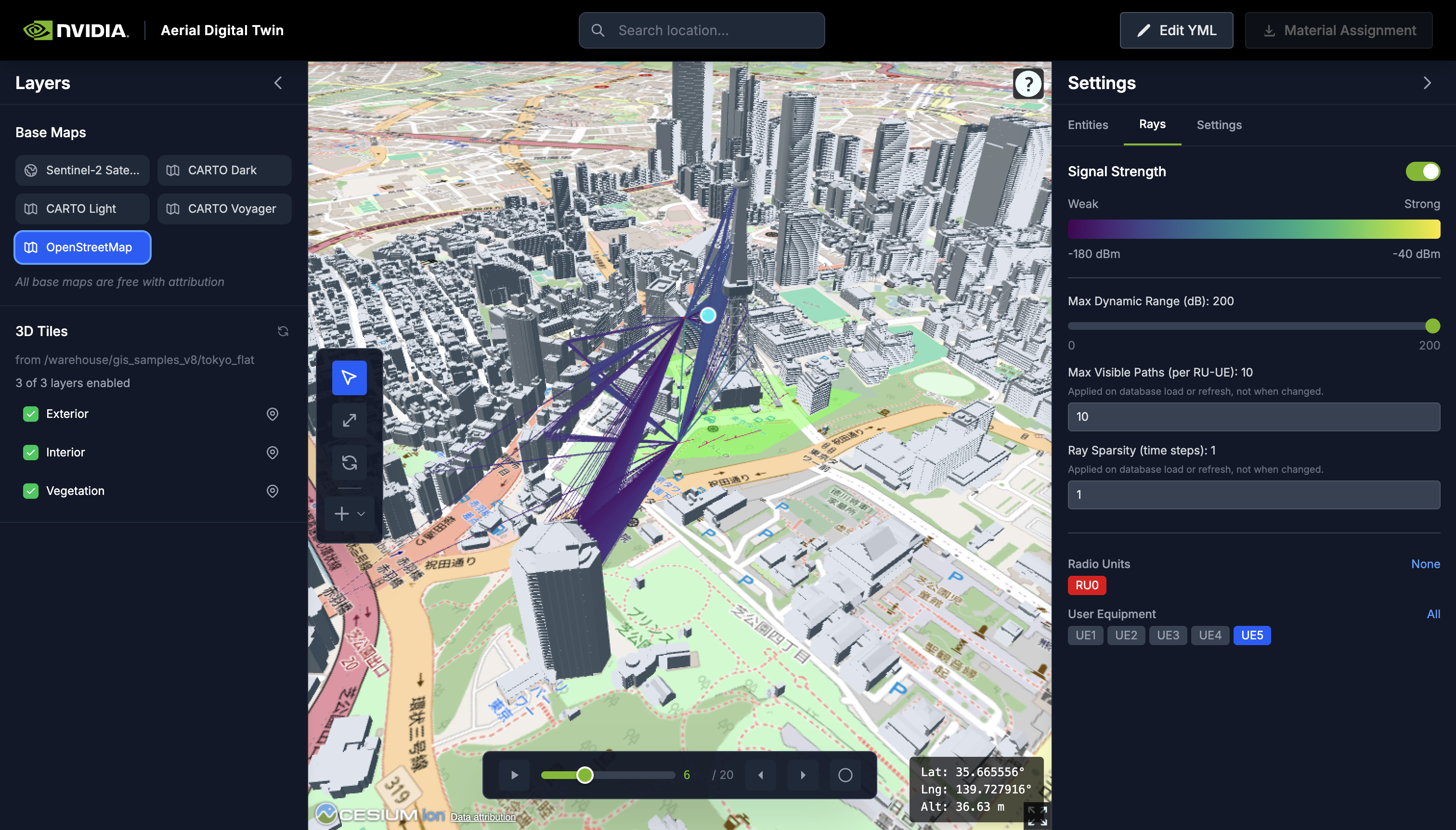
Interpreting Raypaths
Each raypath follows the path geometry recorded by the EM solver — direct, reflected, diffracted, or scattered segments. Color indicates received power in dBm, ranging from dark purple (weaker) to yellow (stronger).
The viewer loads raypaths for antenna element pair (0, 0) only. Other antenna element combinations are not visualized.
Using Dynamic Range
The Max dynamic range slider is the primary tool for interpreting signal coverage. Start with a narrow range (20 to 40 dB) to isolate the strongest paths, then widen it to reveal weaker signals. This helps identify dominant propagation paths and coverage gaps.
RU and UE filter selections are persisted per database namespace, so switching between namespaces restores your previous filter state.
Time-Indexed Data
Each time record in the database includes a global time_idx, batch_idx,
slot_idx, and symbol_idx. UE and scatterer positions update at each time
step, and raypaths are filtered to the current index. Use the timeline to step
through the simulation and observe how signal paths change as entities move.
Select a UE or scatterer in the Entities tab to see its recorded positions as a paginated table with time index, longitude, latitude, and altitude.
Scope
The viewer visualizes ray geometry, received power, entity positions, and 3D building geometry. For tabular result inspection (CIR values, CFR data, exported Parquet fields), see Results and Data.
Related Pages
- See UI for the full viewer layout and workflows.
- See Results Schemas for the Parquet tables produced by simulation runs.
- See Interactive Mode for retrieving CIR results into NumPy during a run.