Controllers | Isaac Lab

Robotic tasks are typically defined in task-space in terms of desired end-effector trajectory, while control actions are executed in the joint-space. This naturally leads to joint-space and task-space (operational-space) control methods. However, successful execution of interaction tasks using motion control often requires an accurate model of both the robot manipulator as well as its environment. While a sufficiently precise manipulator’s model might be known, detailed description of environment is hard to obtain :citesiciliano2009force. Planning errors caused by this mismatch can be overcome by introducing a compliant behavior during interaction.

While compliance is achievable passively through robot’s structure (such as elastic actuators, soft robot arms), we are more interested in controller designs that focus on active interaction control. These are broadly categorized into:

impedance control: indirect control method where motion deviations caused during interaction relates to contact force as a mass-spring-damper system with adjustable parameters (stiffness and damping). A specialized case of this is stiffness control where only the static relationship between position error and contact force is considered.
hybrid force/motion control: active control method which controls motion and force along unconstrained and constrained task directions respectively. Among the various schemes for hybrid motion control, the provided implementation is based on inverse dynamics control in the operational space :citekhatib1987osc.

To provide an even broader set of motion generators, we welcome contributions from the community. If you are interested, please open an issue to start a discussion!

Choosing a controller

Controller	Input command	Output	Required state
`DifferentialIKController`	End-effector position or pose, absolute or relative	Joint position targets	Joint positions, end-effector pose, and Jacobian in a consistent frame
`OperationalSpaceController`	End-effector pose and/or wrench, optionally stiffness and damping ratios	Joint efforts	Jacobian; pose and velocity for motion control; mass matrix for inertial decoupling; gravity vector, contact force, and joint state as required by enabled features

Basic joint-space control sets joint targets directly on the actuators. For joint-space impedance control, use JointImpedanceController (see Joint-space controllers_).

Start with differential IK for reaching or teleoperation with position-controlled actuators. Choose OSC when you need torque commands, task-space compliance, or simultaneous motion and contact force control. For example, wiping a table requires motion along its surface while maintaining a force normal to it.

The IK walkthrough and OSC walkthrough provide complete scenes, state extraction, and runnable demonstrations. Both tutorial scripts use Isaac Sim PhysX and require an Isaac Sim installation.

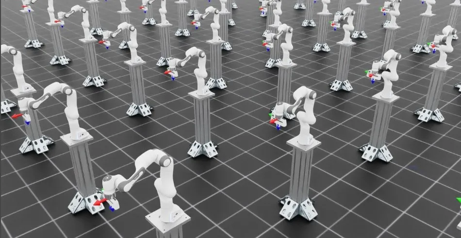
Franka arms on stands with coordinate-frame markers at their end effectors.

IK: reach a pose. Each arm tracks an end-effector goal through joint position targets. Run the IK demonstration to watch the measured and desired frame markers converge.

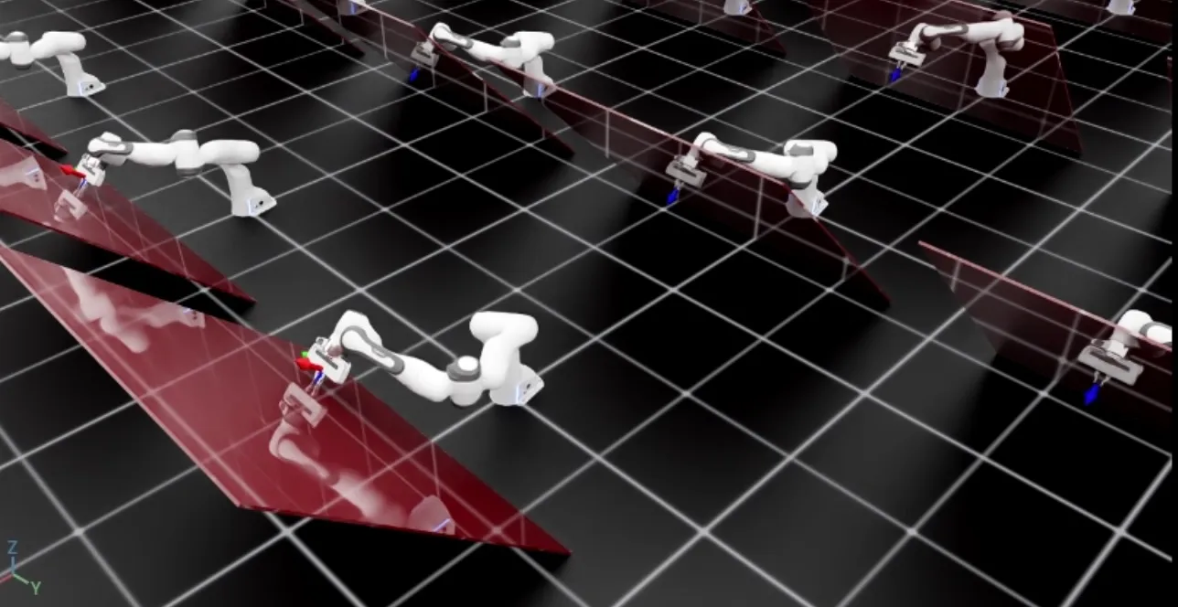
Franka arms touching translucent red tilted walls with their fingertips.

OSC: control motion and contact force. The tilted-wall example commands 10 N along the wall normal while tracking pose in the other directions. Run the OSC demonstration .

The control loop

The IK and OSC instances compute targets from state supplied by the caller; they do not read the simulation or submit actuator commands. ~DifferentialIKController.set_command stores a goal until it is replaced, and every control cycle reads fresh state, calls compute(), stages the targets, and steps the simulation; see Practical API examples for the loop from the IK walkthrough. IK targets are joint positions that the configured position actuator tracks. OSC targets are joint efforts, so configure zero actuator stiffness and damping to keep actuator feedback from adding to them.

Keep the command, end-effector pose, and Jacobian in a consistent coordinate frame. The tutorials use the suffix _b for the robot base frame and _w for the world frame; these names do not transform the data. Absolute poses contain position followed by a quaternion in (x, y, z, w) order. For OSC, commands and axis selections can use a separate task frame, while state passed to compute() remains in the base frame.

Joint-space controllers

There is no dedicated configuration class for selecting a joint-space control mode. Instead, the control mode follows from which targets you set through articulation.actuators: effort targets for torque control, velocity targets for velocity control, and position targets for position control. See Runtime API: articulation.actuators for the runtime API.

Torque control

Action dimensions: "n" (number of joints)

In torque control mode, the input actions are directly set as feed-forward joint torque commands, i.e. at every time-step,

\tau = \tau_{des}

Velocity control

Action dimensions: "n" (number of joints)

In velocity control mode, a proportional control law is required to reduce the error between the current and desired joint velocities. Based on input actions, the joint torques commands are computed as:

\tau = k_d (\dot{q}_{des} - \dot{q})

where $k_d$ are the gains parsed from configuration.

While performing velocity control, in many cases, gravity compensation is required to ensure better tracking of the command. In this case, we suggest disabling gravity for the links in the articulation in simulation.

Position control with fixed impedance

Action dimensions: "n" (number of joints)

In position control mode, a proportional-damping (PD) control law is employed to track the desired joint positions and ensuring the articulation remains still at the desired location (i.e., desired joint velocities are zero). Based on the input actions, the joint torque commands are computed as:

\tau = k_p (q_{des} - q) - k_d \dot{q}

where $k_p$ and $k_d$ are the gains parsed from configuration.

A more complete formulation which considers the dynamics of the articulation would be:

\tau = M \left( k_p (q_{des} - q) - k_d \dot{q} \right) + g

where $M$ is the joint-space inertia matrix of size $n \times n$ , and $g$ is the joint-space gravity vector. This implementation is available through the JointImpedanceController class by setting the impedance mode to "fixed". The gains $k_p$ are parsed from the input configuration and $k_d$ are computed while considering the system as a decoupled point-mass oscillator, i.e.,

k_d = 2 \sqrt{k_p} \times D

where $D$ is the damping ratio of the system. Critical damping is achieved for $D = 1$ , overcritical damping for $D > 1$ and undercritical damping for $D < 1$ .

Additionally, it is possible to disable the inertial or gravity compensation in the controller by setting the flags inertial_compensation and gravity_compensation in the configuration to False, respectively.

Position control with variable stiffness

Action dimensions: "2n" (number of joints)

In stiffness control, the same formulation as above is employed, however, the gains $k_p$ are part of the input commands. This implementation is available through the JointImpedanceController class by setting the impedance mode to "variable_kp".

Position control with variable impedance

Action dimensions: "3n" (number of joints)

In impedance control, the same formulation as above is employed, however, both $k_p$ and $k_d$ are part of the input commands. This implementation is available through the JointImpedanceController class by setting the impedance mode to "variable".

Task-space controllers

Differential inverse kinematics (IK)

Action dimensions: "3" (relative/absolute position), "6" (relative pose), or "7" (absolute pose)

Inverse kinematics converts the task-space tracking error to joint-space error. In its most typical implementation, the pose error in the task-space, $\Delta \chi_e = (\Delta p_e, \Delta \phi_e)$ , is computed as the Cartesian distance between the desired and current task-space positions, and the shortest distance in $\mathbb{SO}(3)$ between the desired and current task-space orientations.

Using the geometric Jacobian $J_{eO} \in \mathbb{R}^{6 \times n}$ , that relates task-space velocity to joint-space velocities, we design the control law to obtain the desired joint positions as:

q_{des} = q + \eta J_{eO}^{-} \Delta \chi_e

where $\eta$ is a scaling parameter and $J_{eO}^{-}$ is the pseudo-inverse of the Jacobian.

It is possible to compute the pseudo-inverse of the Jacobian using different formulations:

Moore-Penrose pseudo-inverse ("pinv"): $A^{-} = A^T(AA^T)^{-1}$ .
Levenberg-Marquardt pseudo-inverse (damped least-squares, "dls"): $A^{-} = A^T (AA^T + \lambda^2 \mathbb{I})^{-1}$ .
Transpose pseudo-inverse ("trans"): $A^{-} = A^T$ .
Adaptive singular-value decomposition (SVD) pseudo-inverse ("svd") from :citebuss2004ik.
Manipulability-aware damped least-squares ("adaptive_dls"): the damping $\lambda$ increases as the Jacobian approaches a singularity.

These implementations are available through the DifferentialIKController class. See ../how-to/run_diff_ik for a runnable example.

Impedance controller

It uses task-space pose error and Jacobian to compute joint torques through mass-spring-damper system with a) fixed stiffness, b) variable stiffness (stiffness control), and c) variable stiffness and damping (impedance control).

Operational-space controller

Similar to task-space impedance control but uses the Equation of Motion (EoM) for computing the task-space force. See ../how-to/run_osc for a runnable example.

Closed-loop proportional force controller

It uses a proportional term to track the desired wrench command with respect to current wrench at the end-effector.

Hybrid force-motion controller

It combines closed-loop force control and operational-space motion control to compute the desired wrench at the end-effector. It uses selection matrices that define the unconstrained and constrained task directions.

Practical API examples

Joint targets

These alternative command examples assume an initialized robot and resolved arm_joint_ids. Each target has shape (num_envs, len(arm_joint_ids)). Set position or velocity feedback gains in the actuator configuration; for direct effort control, set actuator stiffness and damping to zero. See Runtime API: articulation.actuators for the command API and actuators for gains.

Position

Velocity

Effort

joint_pos_target = robot.data.default_joint_pos.torch[:, arm_joint_ids].clone()
robot.actuators.target_command.set_position_index(value=joint_pos_target, joint_ids=arm_joint_ids)
robot.write_data_to_sim()

These calls stage and submit commands. Advance physics and update the scene on each cycle as shown in The control loop.

Task-space goals

The IK walkthrough resets the robot and changes the goal every 150 steps. On intermediate steps, it reads fresh state and computes joint position targets; every step applies the targets and advances the simulation:

if count % 150 == 0:
    # reset time
    count = 0
    # reset joint state
    joint_pos = robot.data.default_joint_pos.torch.clone()
    joint_vel = robot.data.default_joint_vel.torch.clone()
    robot.write_joint_position_to_sim_index(position=joint_pos)
    robot.write_joint_velocity_to_sim_index(velocity=joint_vel)
    robot.reset()
    # reset actions
    ik_commands[:] = ee_goals[current_goal_idx]
    joint_pos_des = joint_pos[:, robot_entity_cfg.joint_ids].clone()
    # reset controller
    diff_ik_controller.reset()
    diff_ik_controller.set_command(ik_commands)
    # change goal
    current_goal_idx = (current_goal_idx + 1) % len(ee_goals)
else:
    # obtain quantities from simulation. The Jacobian DoF axis prepends
    # ``num_base_dofs`` floating-base columns (0 for fixed-base, 6 for
    # floating-base); shift the actuated-joint ids accordingly.
    jacobi_joint_ids = [j + robot.num_base_dofs for j in robot_entity_cfg.joint_ids]
    jacobian = robot.data.body_link_jacobian_w.torch[:, ee_jacobi_idx, :, jacobi_joint_ids]
    ee_pose_w = robot.data.body_pose_w.torch[:, robot_entity_cfg.body_ids[0]]
    root_pose_w = robot.data.root_pose_w.torch
    joint_pos = robot.data.joint_pos.torch[:, robot_entity_cfg.joint_ids]
    # compute frame in root frame
    ee_pos_b, ee_quat_b = subtract_frame_transforms(
        root_pose_w[:, 0:3], root_pose_w[:, 3:7], ee_pose_w[:, 0:3], ee_pose_w[:, 3:7]
    )
    # compute the joint commands
    joint_pos_des = diff_ik_controller.compute(ee_pos_b, ee_quat_b, jacobian, joint_pos)
# apply actions
robot.set_joint_position_target_index(target=joint_pos_des, joint_ids=robot_entity_cfg.joint_ids)
scene.write_data_to_sim()
# perform step
sim.step()
# update sim-time
count += 1
# update buffers
scene.update(sim_dt)

Relative commands also need the measured pose in DifferentialIKController.set_command to resolve the delta at command time.

An OperationalSpaceController instance osc similarly stores its motion/force goal with OperationalSpaceController.set_command, but OperationalSpaceController.compute returns efforts to stage with set_effort_index. Its required state depends on the configured features. Use the IK walkthrough and OSC walkthrough for controller construction, state extraction, and complete repeated loops.

Reactive planners

Typical task-space controllers do not account for motion constraints such as joint limits, self-collision and environment collision. Instead they rely on high-level planners (such as RRT) to handle these non-Euclidean constraints and give joint/task-space way-points to the controller. However, these methods are often conservative and have undesirable deceleration when close to an object. More recently, different approaches combine the constraints directly into an optimization problem, thereby providing a holistic solution for motion generation and control.

Examples of reactive planners include:

RMPFlow (lula): An acceleration-based policy that composes various Reimannian Motion Policies (RMPs) to solve a hierarchy of tasks :citecheng2021rmpflow. It is capable of performing dynamic collision avoidance while navigating the end-effector to a target.
MPC (OCS2): A receding horizon control policy based on sequential linear-quadratic (SLQ) programming. It formulates various constraints into a single optimization problem via soft-penalties and uses automatic differentiation to compute derivatives of the system dynamics, constraints and costs. The MPC formulation for end-effector trajectory tracking in fixed-arm and mobile manipulators described in :citemittal2021articulated considers a kinematic system model with joint limits and self-collision avoidance. See the OCS2 documentation for the external toolbox and examples.

limit throughput in large batches. It also needs the Lula library and robot description files; these dependencies are separate from the selected physics backend.