Manager-Based Workflows#

In the project you generated, the cartpole task is described in env_cfg.py. However, a configuration file is only a description: it never steps the simulation itself. Isaac Lab reads the configuration, builds an environment, and hands each job (applying actions, reading observations, scoring the task) to a helper object called a manager. This lesson shows how those pieces fit together, following the code from Isaac Lab Project Generation all the way to a single call to env.step(actions).

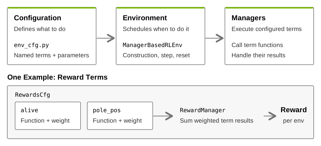
Configuration defines what work to do, the environment schedules when managers run, and managers execute their configured terms. In the reward example, RewardManager combines the weighted alive and pole_pos term results into a reward for each environment. — The configuration describes the work, the environment schedules it, and the managers execute the configured terms and handle their results.#

Use the isaac-lab-workspace/isaac_lab_tutorial project you generated earlier, and open env_cfg.py as you read. You only need to look at the file; you will run the task in the following lessons.

From Configuration to Runtime#

Find BalanceEnvCfg, the class that inherits from ManagerBasedRLEnvCfg. Its fields assemble the scene, actions, observations, events, rewards, and terminations. Its simulation settings also select BalancePhysicsCfg and set the physics time step and the control decimation (how many physics steps happen for each control step).

Think of these classes as a recipe. When Isaac Lab constructs a ManagerBasedRLEnv object, it follows the recipe: it builds the scene, then creates one manager for each job the task needs.

The scene = BalanceSceneCfg(...) field creates an InteractiveScene, which holds the cartpole and its surroundings. Managers look up named assets in this scene. For example, a term can use the SceneEntityCfg to pick out the cart joint from the robot asset. The configuration below selects the joint that connects the slider to the cart:

SceneEntityCfg("robot", joint_names=["slider_to_cart"])

The action, observation, event, reward, and termination fields each configure one manager. A helpful way to remember the split: the configuration says what work to do, and the environment decides when to do it.

Terms Are the Smallest Pieces#

Each manager is built from terms. A term is one small, named piece of the task: a single function (or callable class) plus the parameters it needs. Here is where to find the terms in the cartpole configuration:

Actions: Open ActionsCfg and find the term that targets the cart joint. The ActionManager interprets the incoming action and applies it as a joint effort (a force on the cart).
Observations: Find the policy group in ObservationsCfg. Its terms read joint positions and velocities, which become the policy’s next input.
Events: EventCfg contains reset terms that vary the cart and pole’s initial states, so the policy does not always start from the same pose.
Rewards: RewardsCfg combines weighted terms, such as a survival reward and a pole-angle reward.
Terminations: TerminationsCfg checks the time limit and the cart bounds.

You do not always have to write the functions yourself. The generated balance/mdp/rewards.py holds the task-specific pole-angle reward, while the other terms reuse functions that ship with Isaac Lab.

How Managers Handle Terms#

Each term has a name in its configuration class. For example, these two reward terms are named alive and pole_pos:

@configclass
class RewardsCfg:
    alive = RewardTermCfg(func=mdp.is_alive, weight=1.0)
    pole_pos = RewardTermCfg(
        func=mdp.joint_pos_target_l2,
        weight=-1.0,
        params={
            "asset_cfg": SceneEntityCfg(
                "robot", joint_names=["cart_to_pole"]
            ),
            "target": 0.0,
        },
    )

This excerpt uses the full RewardTermCfg name; the generated file may import it as RewTerm as a common shorthand. The func field identifies the callable (something in Python that you can call, like a function or class with __call__ implemented), params supplies its keyword arguments, and weight controls its contribution to the total reward. The term function receives the environment as its first argument, so it can read the selected asset from env.scene.

Managers handle their terms through three stages:

Prepare: Parse the configuration, validate the term definitions, and resolve scene entity names into joint or body selections. Construct any callable class terms with their configuration and environment.
Execute: When the environment requests the manager’s work, call the relevant terms with the environment and configured parameters. Event terms, for example, run for the requested mode, such as reset or interval.
Reset: Clear the relevant manager buffers and reset stateful terms for the environments whose episodes ended. Other environments can continue using their existing state.

A term can be an ordinary function or a callable class. Class terms can retain state between calls; they inherit from ManagerTermBase and implement the methods their manager requires, including reset behavior when needed.

Each manager handles its term results according to its job:

RewardManager sums weighted contributions into a reward for each environment.
TerminationManager combines Boolean conditions with logical OR, while keeping terminal states and timeouts distinguishable.
ObservationManager organizes signals into groups and can concatenate the terms in each group into a tensor.
ActionManager splits the action vector among its terms, then processes and applies their controls.
EventManager executes operations for the requested event mode.

The environment schedules the managers; each manager executes its configured terms and handles their results.

Base and RL Environments#

ManagerBasedEnv contains the scene, action, observation, and event managers. Its reinforcement learning subclass, ManagerBasedRLEnv, adds reward and termination managers, and can also use command and curriculum managers:

A command manager samples a goal for the robot to track.
A curriculum manager gradually changes the difficulty of the task.

The cartpole task needs neither: its upright target is fixed, and its difficulty does not change during training. Tasks such as walking to a target can use them. The manager API lists every manager and term configuration class.

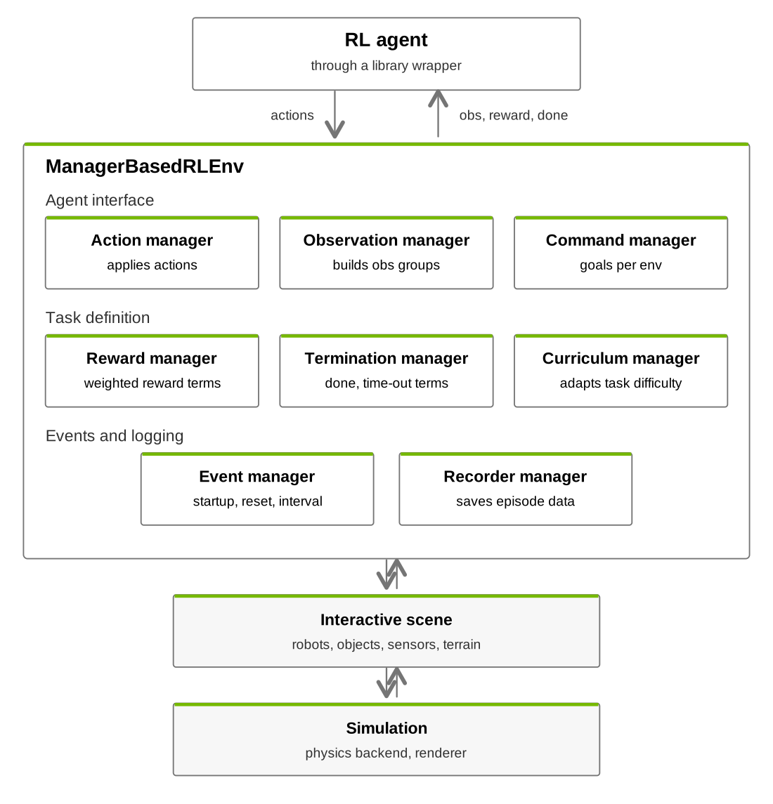
An RL agent exchanges actions and step results with ManagerBasedRLEnv. The environment contains action, observation, command, reward, termination, curriculum, event, and recorder managers, and connects to the interactive scene and simulation. — The manager-based RL environment connects the agent interface and task managers to the interactive scene and simulation.#

Follow One Control Step#

When the agent calls env.step(actions), the environment runs one control step across all of the parallel cartpole environments at once:

ActionManager processes the incoming action once for the control step. It applies the resulting control before each physics substep.
The selected physics backend advances the scene. The cartpole configuration uses a decimation of two, so one control step advances two physics steps.
The RL environment evaluates the reward and termination terms. An environment that reaches its time limit or cart bound ends its episode, and reset events prepare its next initial state.
ObservationManager supplies the next policy observation. The step also returns the reward, terminated, truncated, and an information dictionary.

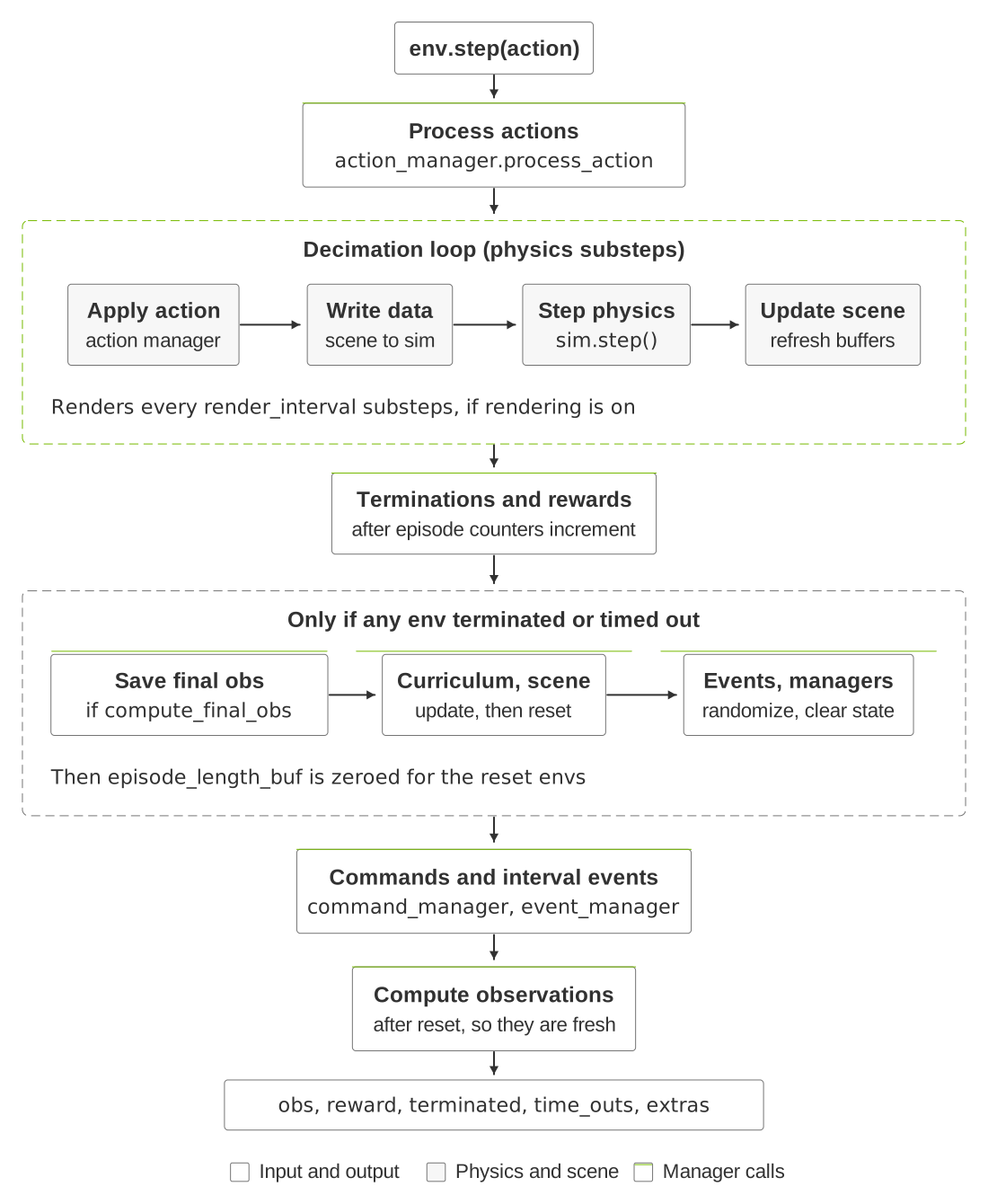
A call to env.step processes the action, applies it across physics substeps, evaluates terminations and rewards, resets affected environments, updates commands and events, computes fresh observations, and returns the step results. — One manager-based environment step, including the physics substeps and the reset path for environments that have ended an episode.#

To learn more about any detail of this sequence, see the ManagerBasedRLEnv.step API reference.

Every term works on a batch of environments, so one step() call can advance many independent cartpoles. One cartpole can reset while the others keep going. Notice also that the action is processed once per control step but applied before every physics step. That is why decimation matters: it sets how long each action is held.

Default Configuration and Overrides#

You can run a task without choosing every setting yourself. The task’s configuration gives you a starting point, including a default physics backend. In the generated cartpole project, look for this line in BalanceEnvCfg’s __post_init__() method:

self.sim.physics = BalancePhysicsCfg()

BalancePhysicsCfg lists the task’s physics choices and sets Newton with MJWarp as the default. The key line is default = newton_mjwarp. Here is an abbreviated view of the configuration, with the backend settings omitted so you can focus on how the default is selected:

@configclass
class BalancePhysicsCfg(PresetCfg):
    newton_mjwarp: NewtonCfg  = NewtonCfg(...)
    ovphysx      : OvPhysxCfg = OvPhysxCfg(...)
    default = newton_mjwarp

newton_mjwarp names a configured backend option. Assigning that configuration to default makes it the choice Isaac Lab uses when you do not supply a physics selector. (The ellipses ... above are placeholders.)

If you run the command below, Isaac Lab uses that default automatically:

uv run isaaclab random_agent               \
  --task IsaacLabTutorial-Balance-Cartpole \
  --visualizer none

To try another backend, add a physics selector to your command. For example, this command runs the same task with OV PhysX:

uv run --extra ovphysx isaaclab random_agent \
  --task IsaacLabTutorial-Balance-Cartpole   \
  --visualizer none                                 \
  physics=ovphysx

There are two parts to that change: --extra ovphysx makes the integration available, and physics=ovphysx tells the task to use it for this run. You can try a different backend this way without editing env_cfg.py. Each task has its own available choices. To see yours, use the help or preset listing introduced in The Isaac Lab CLI.

Before building the environment, Isaac Lab settles on the configuration for your run: the task’s default, with any overrides you supplied. It then creates the matching PhysicsManager and the backend’s versions of the assets and sensors. Once the scene is ready, the task managers resolve their terms against it—for example, finding the cart joint that an action term will control.

Review#

Check Your Understanding#

How do you calculate the control interval from the physics time step and decimation?

Apply What You Learned#

How would you trace one cartpole control step through the configured managers and physics substeps? Distinguish action processing from application, identify the manager operations, and calculate the control interval from the configuration.

Key Takeaways#

Configuration classes declare task terms; managers execute them.
A control step may include several physics substeps.
The physics backend advances the scene; rendering produces images when needed.

Resources#

Isaac Lab Managers API — API reference for manager classes, term configurations, and scene entity selection.
Creating a Manager-Based Base Environment — A guide to configuring a scene, actions, observations, and events in a manager-based environment.
Creating a Manager-Based RL Environment — A guide to adding rewards, termination conditions, and other reinforcement learning components to a manager-based environment.
Backend Architecture — An explanation of backend selection, common simulation interfaces, and the physics manager lifecycle.