

Cartpole Training#
This is the behavior you will work toward: balancing after a reset. The video is a reference run; your results depend on your training conditions.#
In the previous lesson, you verified task registration and observed zero-action and random-action behavior. Now let’s use the same task to train a policy with Proximal Policy Optimization (PPO), a popular reinforcement learning algorithm, inspect its training metrics, and compare saved checkpoints with those baselines.
You’ll start with a short training session, then run training with the generated project’s default settings. You’ll use the plots and recordings together to see what improved and how well the policy performs under the conditions you tested.
Note
Before you begin, complete the baseline checks in The Cartpole
Example. Run every command in this lesson from
the same generated isaac-lab-workspace/isaac_lab_tutorial root. Keep the task
and PPO configuration unchanged so you can follow the comparisons below.
Choose a Starting Environment Count#
Start with 64 environments for the short run below. The generated default
run uses 4,096, which you can try if your GPU has enough memory and you have
time for a longer training session. Training needs room in GPU
memory for rollouts, networks, and optimizer state alongside the simulation. If
you run out of GPU memory, lower --num_envs and try again.
Optional: Compare Runtime Throughput Before a Larger Run
Use the Isaac Lab benchmarking guide if you want to tune the environment count. Compare candidate counts with the same task, backend, seed, and measurement settings. Look for a count that gives good overall throughput while leaving memory for training. Try a short training run with that count before committing to a longer run.
A runtime benchmark measures environment stepping. It excludes the policy updates and rollout storage needed during training, so use its fastest count as a starting point rather than a final choice.
With 16 steps per rollout, 64 environments collect 1,024 transitions per PPO iteration; 4,096 collect 65,536. This changes the amount of training experience, so compare runs by environment transitions as well as iterations.
Train a Policy#
We’ll start with a short PPO training session and use --visualizer none to avoid the
extra work of displaying a live simulation view while the policy trains:
Try a short session to check that training works.
uv run isaaclab train                      \
  --rl_library rsl_rl                      \
  --task IsaacLabTutorial-Balance-Cartpole \
  --num_envs 64                            \
  --max_iterations 50                      \
  --seed 42                                \
  --run_name cartpole_short                \
  --visualizer none
Here’s what the options do:
--rl_library rsl_rlselects RSL-RL to perform PPO updates.--taskselects the registered cartpole environment.--num_envs 64and--max_iterations 50set the short run’s size/duration.--seed 42sets the random seed.--run_name cartpole_shortlabels the saved run.--visualizer nonetrains without drawing a live viewer.
The training log’s ETA gives you an idea of how long the run will take on your machine.
This command uses
PPORunnerCfgfromrsl_rl_ppo_cfg.py. At each iteration, the policy collects a rollout from the environments, computes returns and advantages, and updates the actor (the policy) and critic (the value estimator) from mini-batches of that experience.This short run collects 51,200 environment transitions: 64 environments × 16 steps per rollout × 50 iterations. It gives you an initial training run and saved checkpoints to inspect. To explore the training settings, look for the configuration file
logs/.../params/agent.yamlusingfind.Next, use the defaults for a longer run with more parallel environments:
uv run isaaclab train                      \
  --rl_library rsl_rl                      \
  --task IsaacLabTutorial-Balance-Cartpole \
  --seed 42                                \
  --run_name cartpole_default              \
  --visualizer none
The two runs use the same task and seed, but use different numbers of parallel environments and amounts of training experience. Here’s a summary of the reference runs to help you compare them:
Setting |
Short run |
Full run |
|---|---|---|
Run name |
|
|
Parallel environments |
64 |
4,096 |
PPO iterations |
50 |
150 |
Steps per rollout |
16 |
16 |
Environment transitions |
51,200 |
9,830,400 |
Analyze the Results#
Let’s look at the results from three angles:
Terminal metrics: inspect the final reward terms and episode endings.
Learning curves: compare progress over the full training run in TensorBoard.
Policy playback: watch whether the saved policy actually balances the pole.
Inspect the Terminal Metrics#
Your terminal prints progress as training runs. Here’s the final output from the reference run, which you can compare with your own:
Learning iteration 149/150

                               Run name: cartpole_default
                            Total steps: 9830400
                       Steps per second: 824669
                        Collection time: 0.038s
                          Learning time: 0.041s
                        Mean value loss: 0.0000
                    Mean surrogate loss: 0.0047
                      Mean entropy loss: -1.1233
                            Mean reward: 4.94
                    Mean episode length: 300.00
                        Mean action std: 0.08
                   Episode_Reward/alive: 1.0000
             Episode_Reward/terminating: 0.0000
                Episode_Reward/pole_pos: -0.0074
                Episode_Reward/cart_vel: -0.0032
                Episode_Reward/pole_vel: -0.0014
           Episode_Termination/time_out: 1.0000
 Episode_Termination/cart_out_of_bounds: 0.0000
--------------------------------------------------------------------------------
                         Iteration time: 0.08s
                           Time elapsed: 0:00:12
                                    ETA: 0:00:00

Training time: 12.67 seconds
Start with these clues when reading the output:
The final logged metrics are consistent with episodes reaching the 300-step time limit: mean episode length is 300, the timeout rate is 1.0, and the cart-out-of-bounds rate is 0.0.
The mean reward of 4.94 is close to the maximum implied by the logged terms: the policy receives the full alive reward while keeping the pole-angle, cart-velocity, and pole-velocity penalties small.
Together, these values are consistent with a policy that balances the pole for the full five-second episode rather than merely avoiding an early termination.
The optimization statistics also look stable at the end of this run. The value loss is near zero, the surrogate loss is small, and the action standard deviation has fallen to 0.08. These values describe the final PPO updates; to judge balancing, also check the task metrics and watch the policy.
Inspect the Learning Curves#
RSL-RL writes the resolved configuration, event data, and checkpoints below
logs/rsl_rl/.
Find your run directories and saved checkpoints:
find logs/rsl_rl -maxdepth 3 -type d -print
find logs/rsl_rl -name 'model_*.pt' -print
Open the training curves in TensorBoard.
Start TensorBoard in the project root with the log directory as its data source:
uv run tensorboard --logdir logs/rsl_rl
If TensorBoard is running on a remote machine, you can forward the port to your local machine. From a terminal on your local machine, forward the port listed by the
tensorboardcommand over SSH:ssh -N -L PORT:localhost:PORT USER@REMOTE_HOST
Replace
PORTwith the port number printed by thetensorboardcommand, and replaceUSER@REMOTE_HOSTwith your SSH user and the hostname or IP address of the remote machine. Keep the SSH session open, then visit the link given by thetensorboardcommand in your local browser.
In the next section we’ll show you how to compare runs with Weights & Biases, but first let’s look at the TensorBoard metrics. Here are some suggestions for what to look for in TensorBoard:
Check
Train/mean_episode_lengthandTrain/mean_reward. The mean reward should increase and the mean episode length should approach the maximum of 300 steps.Check
Episode_Termination/cart_out_of_boundsandEpisode_Termination/time_out. The cart-out-of-bounds rate should decrease to zero, and the timeout rate should increase to one.Check
Episode_Reward/cart_velandEpisode_Reward/pole_vel. These values should trend toward zero, indicating that the policy is keeping the cart and pole stable.
You can also use the TensorBoard logs to make your own plots later. For now, compare your curves with the reference figure below. It shows reward and episode length for both runs, with environment transitions on a logarithmic axis.
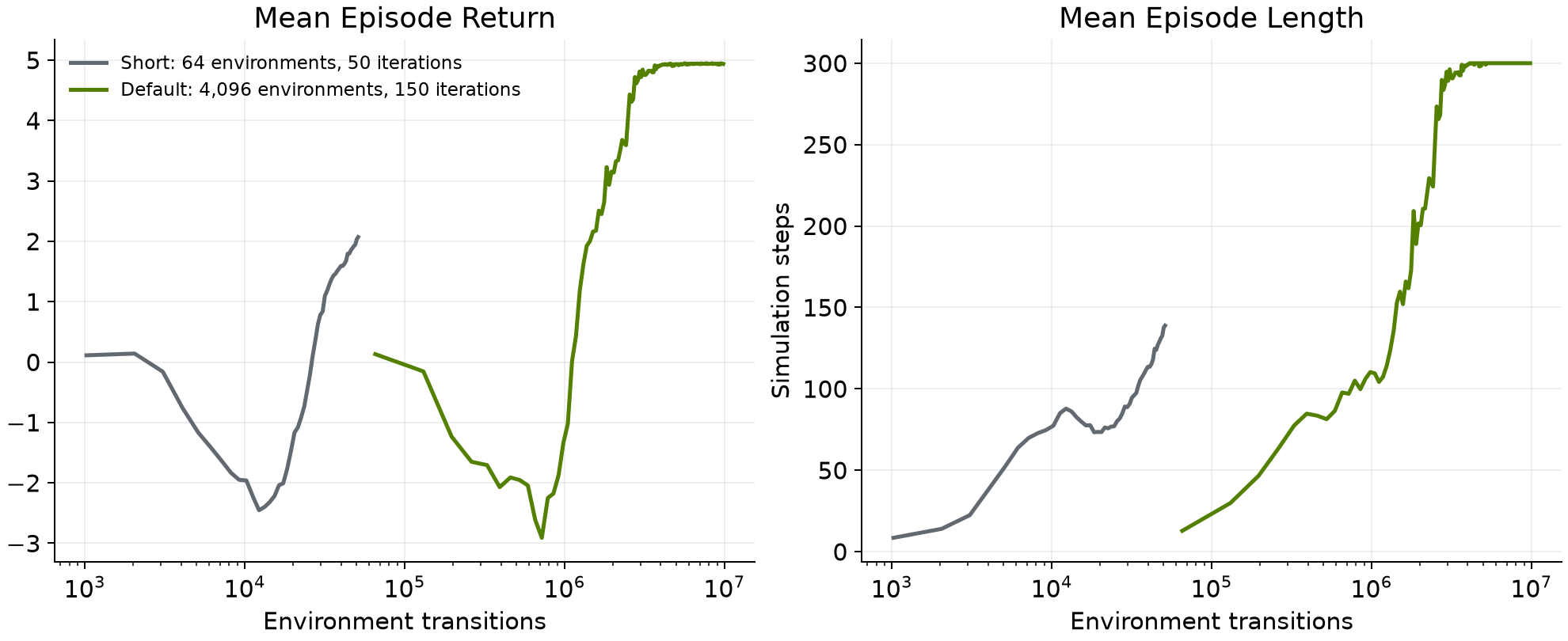
Reference reward and episode-length curves from the TensorBoard logs.#
Compare Runs With Weights & Biases#
If you’d like interactive charts and an easy way to compare experiments, try Weights & Biases (W&B). Isaac Lab includes support for a W&B logger, so you can record metrics and the resolved configuration without writing a plotting script.
The generated project includes W&B as an optional dependency. If you have a W&B account, enable this extra and authenticate on the machine where you train. Run this command from the generated project root:
uv run --extra wandb --with wandb==0.26.1 wandb login
Include --extra wandb in each W&B command below so uv installs the project’s
optional W&B dependencies. The additional --with wandb==0.26.1 constraint
keeps the wandb.util.generate_id API used by this Isaac Lab logger; newer W&B
releases remove that API.
Follow the prompt to enter your W&B API key. If you use a team project, set
WANDB_USERNAME to the team entity name before training; the RSL-RL logger uses
this variable to choose the W&B entity.
To try W&B, use the two training commands below instead of the earlier ones. If you’ve already finished those runs, you can keep using TensorBoard or start new runs with W&B. These commands won’t import your existing TensorBoard logs.
uv run --extra wandb --with wandb==0.26.1 isaaclab train \
  --rl_library rsl_rl                                    \
  --task IsaacLabTutorial-Balance-Cartpole               \
  --num_envs 64                                          \
  --max_iterations 50                                    \
  --seed 42                                              \
  --run_name cartpole_short                              \
  --logger wandb                                         \
  --log_project_name cartpole-training                   \
  --visualizer none

uv run --extra wandb --with wandb==0.26.1 isaaclab train \
  --rl_library rsl_rl                                    \
  --task IsaacLabTutorial-Balance-Cartpole               \
  --seed 42                                              \
  --run_name cartpole_default                            \
  --logger wandb                                         \
  --log_project_name cartpole-training                   \
  --visualizer none
Open the project link printed by W&B in your browser. Select the two runs in the
cartpole-training project and compare Train/mean_reward,
Train/mean_episode_length, and the reward and termination metrics listed
above. The run names include a timestamp followed by the --run_name suffix.
The W&B logger also writes TensorBoard event files and saves checkpoints under
logs/rsl_rl/, so the TensorBoard and playback commands still apply.
The two runs collect different amounts of experience per iteration: 1,024 transitions for the short run and 65,536 for the default run. Keep that difference in mind when comparing curves. The reference figure above instead plots both runs against environment transitions, with episode length in simulation steps.
If the training machine cannot connect to W&B, prefix each training command
with WANDB_MODE=offline. W&B prints the local run directory; upload it later
from a machine with network access using:
uv run --extra wandb --with wandb==0.26.1 wandb sync PATH_TO_OFFLINE_RUN
Replace PATH_TO_OFFLINE_RUN with the directory printed by W&B.
Compare the Saved Policies#
Now for the most important analysis: watching what your policies have learned.
The isaaclab play command can run a saved policy and record a video.
The recording command uses Newton GL. RTX is optional and depends on compatible ovrtx plugins.
CARTPOLE_CHECKPOINT=$(find logs/rsl_rl                   \
  -path '*cartpole_short/model_49.pt' -print -quit)

uv run --with 'moviepy<2'                                \
  isaaclab play                                          \
  --rl_library rsl_rl                                    \
  --task IsaacLabTutorial-Balance-Cartpole               \
  --checkpoint "$CARTPOLE_CHECKPOINT"                    \
  --num_envs 16                                          \
  --seed 123                                             \
  --visualizer newton                                    \
  --video --video_length 900                             \
  env.sim.default_visualizer_cfg.eye='[14.0,-18.0,13.0]' \
  env.sim.default_visualizer_cfg.lookat='[0.0,0.0,0.8]'  \
  env.sim.default_visualizer_cfg.focal_length=24.0
The shell variable CARTPOLE_CHECKPOINT holds the checkpoint path, so you can
reuse the playback command by changing that path. The playback command loads
the policy without further training and records 900 control steps (15 seconds).
By default, the video is written to a videos subdirectory of the checkpoint’s
parent directory. You can find the recording with:
find "$(dirname "$CARTPOLE_CHECKPOINT")/videos" -type f -name '*.mp4'
Playback of the 50-iteration checkpoint.#
Now locate and record the final checkpoint from the default run:
CARTPOLE_CHECKPOINT=$(find logs/rsl_rl \
  -path '*cartpole_default/model_149.pt' -print -quit)

# This is the same command as above, but with the new checkpoint path.
# You can use your shell history to repeat the command.
uv run --with 'moviepy<2'                                \
  isaaclab play                                          \
  --rl_library rsl_rl                                    \
  --task IsaacLabTutorial-Balance-Cartpole               \
  --checkpoint "$CARTPOLE_CHECKPOINT"                    \
  --num_envs 16                                          \
  --seed 123                                             \
  --visualizer newton                                    \
  --video --video_length 900                             \
  env.sim.default_visualizer_cfg.eye='[14.0,-18.0,13.0]' \
  env.sim.default_visualizer_cfg.lookat='[0.0,0.0,0.8]'  \
  env.sim.default_visualizer_cfg.focal_length=24.0

find "$(dirname "$CARTPOLE_CHECKPOINT")/videos" -type f -name '*.mp4'
Using the same environment count, seed, viewer, and recording length makes the two checkpoint videos directly comparable.
Playback of the 150-iteration checkpoint.#
Compare your recordings with the zero-action and random-action baselines from the previous lesson. In the reference recordings shown here, the short checkpoint usually keeps the poles near upright but can let carts drift toward the track boundary. The default checkpoint recovers more consistently from randomized resets and keeps both pole angle and cart position controlled. Together with the reward and episode-length curves, the recordings support learning progress for this seed. To find out how consistently the policy performs, you’d need to try additional training seeds or changes to the dynamics.
Review#
Check Your Understanding#
Does one successful playback recording prove that a policy is reliable?
Answer
No. One recording shows a limited set of attempts under particular conditions. Additional complete-episode evaluations and seeds help assess consistency.
Apply What You Learned#
How would you use your training metrics and checkpoint playback to judge learning progress and choose a further reliability check? Compare the trained policies with zero-action and random-action baselines, and describe what another seed or evaluation could tell you.
Agent Tutor Prompt
Copy this prompt and include your answer:
Review my answer to this question: How would you use your training metrics and checkpoint playback to judge learning progress and choose a further reliability check? Compare the trained policies with zero-action and random-action baselines, and describe what another seed or evaluation could tell you.
My answer: [paste your answer here].
Check my reasoning about baselines, pole angle, cart drift, episode endings, training experience, and additional seeds. Ask for missing context rather than assuming it. Identify what I explained well, point out one gap or misconception, and ask a follow-up question that helps me improve my answer. Let me revise it before supplying a complete answer.
Key Takeaways#
Start with a short run, then try a longer one once training works.
Environment count changes both workload and experience collected per iteration.
Use metrics and playback together, comparing them with your baselines to understand what the policy learned.
Resources#
Isaac Lab Reinforcement Learning — Documentation on supported reinforcement learning libraries and workflows for training and evaluating policies.
RSL-RL — An overview of the GPU-based reinforcement learning library used for robot policy training.
W&B Login — Authenticate the training machine with W&B.
W&B Sync — Upload runs recorded in offline mode.