Generates a synthetic dataset of arbitrary size from a small sample of a real dataset, for benchmarking vector indexes at scales (100M, 1B, 10B+) where the real dataset isn’t available at the target size. Purely random vectors aren’t a substitute — the clustering structure, neighbor density, and intrinsic dimensionality of real embeddings are what dominate ANN index behavior, and random data has none of those.

The synthetic dataset approximates the real dataset’s behavior under ANN search rather than its raw vector content. When you build the same index on both and sweep the same search-effort knob (CAGRA’s itopk_size, HNSW’s efSearch, DiskANN’s L, …), the recall–throughput Pareto curves track each other and relative algorithm rankings carry over.

Ground truth is generated alongside the data and can be computed at any target size without storing the full dataset on disk. See How it works for the mechanism.

When to use this

Use it when:

• You want to benchmark a vector index at 100M / 1B / 10B+ but only have a small (~10M) real dataset.
• You want benchmark numbers (recall, throughput, build time) on the synthetic data that carry over to what you’d see on the real data at the same scale.
• The real dataset is sensitive or proprietary and can’t be shared, but you want a collaborator (or vendor) to benchmark a vector index against something representative of it. Fit a fingerprint locally and share that small file (.npz) instead of the dataset — it stores only per-cluster aggregate statistics, never raw rows. The collaborator regenerates the synthetic dataset locally. See How it works for what’s in the fingerprint.

Don’t use it when:

• You want to use the data for anything other than ANN-index benchmarking — training or fine-tuning embedding models, evaluating downstream ML tasks, distance-correctness tests against a real reference, or any workload that depends on the actual vector content. The synthetic vectors only preserve index-search behavior; they aren’t a substitute for the real dataset in any other context.

How it works

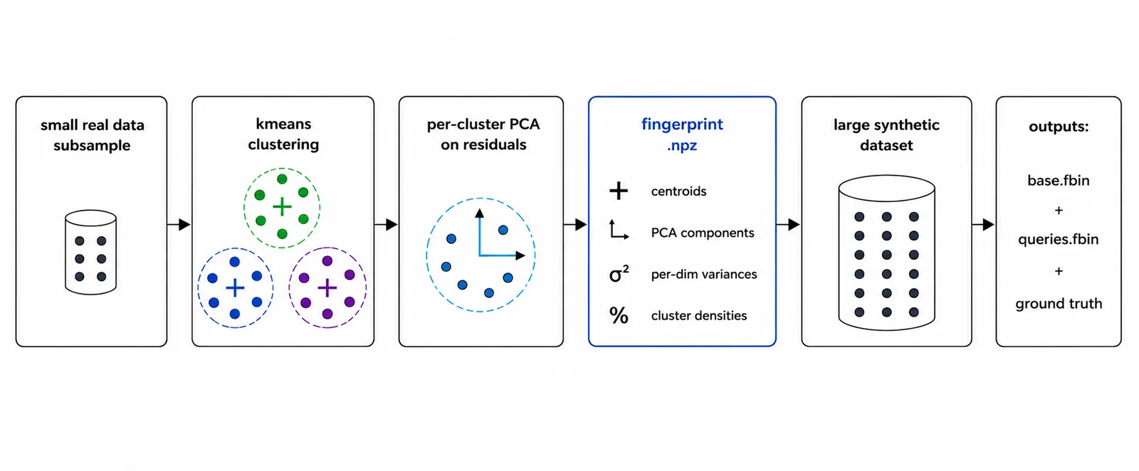
The fit step learns the small fingerprint highlighted in blue above. The generate step turns the fingerprint into a synthetic dataset of arbitrary size, and ground truth is computed alongside it: each query probes its nprobes nearest clusters, those clusters are regenerated deterministically from the fingerprint, and brute-force k-NN is run against just those candidates. This is what makes 10B+ scale GT tractable. Note that nprobes here is an internal parameter of the GT pipeline (how many clusters we probe to find true neighbors), not a search-time parameter of any specific ANN index.

What the fingerprint contains

The fit step produces a single NPZ file holding only per-cluster aggregate statistics:

• centroids — means over each cluster’s points.
• pca_components_arr — eigenvectors of the per-cluster residual covariance (linear functionals of the cluster, not raw rows).
• pca_explained_var_arr, pca_noise_var — eigenvalues and residual variance scalars.
• pca_n_components — the requested number of PCA components.
• variances_per_dim — per-dim variance per cluster.
• densities — per-cluster point counts, normalized.
• norm_unit — single bool: whether the fit-time input was (≈) L2-unit-norm.
• norm_quantiles — per-cluster norm inverse-CDF: a (n_clusters, 256) grid of the real vector-norm distribution within each cluster. At generate time each vector draws a target norm from its cluster’s grid (inverse-CDF sampling), so the synthetic data reproduces each cluster’s real radial spread.

No individual row of the original data is stored anywhere in the fingerprint, and the synthetic data emitted at generate-time is centroid + RNG, never a copy of a real row.

Query generation (random jitter)

Queries are sampled from the dataset itself and perturbed with a small Gaussian, so they sit on the data manifold without being exact-match copies of database rows. The generate step produces them automatically alongside base.fbin and GT.

If you also have the real dataset and want matching queries on it (e.g. for the synth-vs-real comparison in Step 6), run cuvs_bench.generate_groundtruth --queries random-jitter on it.

Installation

Install cuvs_bench following the cuvs-bench installation guide, then add the synthesize_dataset extra to pull in the additional dependencies:

$
pip install 'cuvs_bench[synthesize_dataset]'

A GPU is required. CPU-only operation isn’t supported.

Step-by-step

Step 1 — Pick sample_size, n_clusters, and ncomp

Two raw sizes feed the recipe:

• total_rows — target size of the synthetic dataset you want to generate (e.g. 100M, 1B, 10B etc).
• sample_size — size of the real-data slice you fit the fingerprint on (passed to fit).

Three knobs are derived from (or chosen alongside) those:

• SF (scale factor) = total_rows / sample_size — how much we stretch the fitting sample to reach the target size.
• PPC (points per cluster) = sample_size / n_clusters — average number of real sample points per KMeans cluster.
• ncomp — number of PCA components fit per cluster, i.e. the rank of the low-rank Gaussian sampler used to draw synthetic points around each centroid.

Use the recommended defaults: SF=100, PPC=100, ncomp=32. With those fixed, the only thing you choose is the target size, and everything else follows mechanically:

sample_size = target_size / 100        # SF = target_size / sample_size = 100
n_clusters  = sample_size / 100        # PPC = sample_size / n_clusters  = 100
ncomp       = 32                       # good middle ground at PPC=100

So for a 100M target: sample_size=1M, n_clusters=10K, ncomp=32. For a 1B target: sample_size=10M, n_clusters=100K, ncomp=32.

ncomp=32 is the default because it sits in the empirical sweet spot at PPC=100 — large enough to capture the dominant intra-cluster correlations on typical embedding data, small enough to estimate reliably with 100 points per cluster. Above the ceiling listed below, recall degrades uniformly across the entire recall range; below ~16 the model is under-expressive at large target sizes.

Step 2 — Fit the cluster fingerprint

$
python -m cuvs_bench.synthesize_dataset fit \
>
    --dataset /path/to/your_real_data.fbin \
>
    --sample_size 1000000 \
>
    --n_clusters 10000 \
>
    --pca_components 32 \
>
    --output fingerprint.npz

The output fingerprint.npz can be reused for any target size.

Supported input formats: .fbin (cuvs-bench layout), .npy, .pkl.

Step 3 — (Recommended) Verify nprobes at small scale

nprobes is how many nearest clusters each ground-truth query probes when computing GT. We don’t search the whole synthetic dataset for each query — that would be O(total_rows) per query and takes long at multi-billion scale. Instead, for each query we re-generate only the nprobes clusters whose centroids are closest to the query and run brute-force k-NN against just those points.

By construction nprobes ≤ n_clusters (probing more clusters than exist is meaningless). Recommended starting point: nprobes ≈ 5% of n_clusters. For the fit recipe in Step 1 (n_clusters=10K at 100M targets, 100K at 1B), that lands at nprobes=500 and 5000 respectively. Empirically this keeps Step 3’s recall above 0.999, i.e. the cheap nprobe GT and the exact GT agree on more than 99.9% of true neighbors. Higher nprobes is more accurate but linearly more expensive at GT time.

What “recall” means in this step. The recall reported by verify is internal to the GT pipeline — it measures how well the cheap nprobe GT agrees with the exact streaming GT. It is not the recall of any ANN index you’ll later benchmark on the synthetic data.

nprobes requirements shrink with total_rows, not grow. A fingerprint has a fixed n_clusters, so at larger total_rows each cluster holds proportionally more points (same densities, just more samples each). For a fixed k, a query’s top-k true neighbors then concentrate in fewer nearby clusters than they would at a smaller scale — both because each cluster contributes more candidates and because the k-th nearest distance shrinks as overall density grows. So an nprobes calibrated at a small total_rows is a safe upper bound for the same fingerprint at larger target sizes — it can only over-probe at the larger scale, never under-probe.

Before paying for the full-scale generation, run the cheap nprobe GT against the exact streaming GT at a small total_rows and check that they agree:

$
python -m cuvs_bench.synthesize_dataset verify \
>
    --fingerprint fingerprint.npz \
>
    --total_rows 1000000 \
>
    --n_queries 1000 \
>
    --k 10 \
>
    --nprobes 500            # ~5% of n_clusters=10K

If GT-vs-GT recall ≥ 0.999, that nprobes is safe to reuse in Step 4 at any larger total_rows — Step 3 conservatively over-estimates what you actually need at scale, so the value carries over without re-tuning. If recall is lower, bump nprobes and re-run Step 3 (cheap).

Step 4 — Generate the synthetic dataset + queries + GT

Option 1 (Fast path): nprobe GT.

Uses the nprobes you settled on in Step 3 — only the nprobes clusters nearest each query are regenerated and brute-forced. As mentioned in the previous step, using about 5% of n_clusters is a good heuristic to reach ≥ 0.999.

$
python -m cuvs_bench.synthesize_dataset generate \
>
    --fingerprint fingerprint.npz \
>
    --total_rows 1000000000 \
>
    --n_queries 10000 \
>
    --k 10 \
>
    --nprobes 500 \
>
    --gt_mode nprobe \
>
    --output_dir synthetic_100M/

Option 2 (Exact path, slower): exact GT.

Set --gt_mode exact for exact GT — every cluster is regenerated on the GPU and brute-forced against the queries. Slower than the nprobe path, but still faster than a standard GT computation at the same total_rows because there’s no disk I/O or host↔device transfer of the dataset.

$
python -m cuvs_bench.synthesize_dataset generate \
>
    --fingerprint fingerprint.npz \
>
    --total_rows 1000000000 \
>
    --n_queries 10000 \
>
    --k 10 \
>
    --gt_mode exact \
>
    --output_dir synthetic_100M/

Outputs (cuvs-bench-compatible):

• synthetic_100M/base.fbin
• synthetic_100M/queries.fbin
• synthetic_100M/groundtruth.neighbors.ibin
• synthetic_100M/groundtruth.distances.fbin
• synthetic_100M/dataset.yaml — dataset registry entry, ready to pass to --dataset-configuration

Disk-size note. base.fbin is materialized to disk at full total_rows × ncols × 4 bytes. Make sure --output_dir lives on a volume with enough free space before kicking off a large run. Generation streams cluster-by-cluster directly to disk, so host RAM stays bounded (~a few GB) regardless of total_rows — only the disk volume matters.

Step 5 — Benchmark and plot

Move synthetic_100M/ under your dataset root so --dataset-path is its parent, then run the cuvs bench algorithms to produce a recall-vs-throughput (or recall-vs-latency) Pareto plot. Any algorithm supported by cuvs_bench works here — see the full list of supported algorithms.

$
python -m cuvs_bench.run \
>
    --dataset synthetic_100M \
>
    --dataset-path $RAPIDS_DATASET_ROOT_DIR \
>
    --dataset-configuration $RAPIDS_DATASET_ROOT_DIR/synthetic_100M/dataset.yaml \
>
    --algorithms cuvs_cagra,cuvs_ivf_pq,hnswlib,diskann_memory \
>
    --build --search
$
$
python -m cuvs_bench.plot \
>
    --dataset synthetic_100M \
>
    --dataset-path $RAPIDS_DATASET_ROOT_DIR \
>
    --algorithms cuvs_cagra,cuvs_ivf_pq,hnswlib,diskann_memory \
>
    --output-filepath ./plots/

The run drops results under $RAPIDS_DATASET_ROOT_DIR/<dataset_name>/result/{build,search}/... as JSON + auto-exported CSV. The plot is one PNG per dataset.

Step 6 — (Optional validation) Compare against the real dataset

If you also have the real dataset at the same total_rows, you can validate that the synthetic-data benchmark numbers are a faithful stand-in for the real ones. If the synthetic dataset is built with the right parameters, both curves should overlap closely across the algorithms you ran. Repeat Step 5 with the real dataset, then compare.

Use random-jitter queries on the real dataset too. The synthetic dataset’s queries are random-jitter by construction (sampled from the data and perturbed with a small Gaussian — see Query generation), so the synthetic benchmark already measures index behavior under a data-query distribution where queries sit on the data manifold. To make the real-vs-synth comparison apples-to-apples, the real dataset’s queries should follow the same scheme — otherwise you’d be comparing two different query distributions on top of two different data distributions, and any gap in the curves could be either effect. Generate them with:

$
python -m cuvs_bench.generate_groundtruth \
>
    /path/to/your_real_data.fbin \
>
    --queries=random-jitter \
>
    --n_queries=10000 \
>
    --k=10 \
>
    --output=$RAPIDS_DATASET_ROOT_DIR/my_real_data

This writes queries.fbin, groundtruth.neighbors.ibin, and groundtruth.distances.fbin into the real dataset’s directory; reference those as query_file / groundtruth_*_file in the YAML below.

If the real dataset already ships with a fixed benchmark query set you specifically want to evaluate on, you can use that instead — but the comparison is then no longer a clean test of the data-distribution match alone, so you’ll likely need to re-tune the synthetic fingerprint (loop back to Step 1). Do the tuning at parity — generate the synthetic dataset at the same total_rows as the real dataset, plot real-vs-synth, and adjust the knobs until the curves overlap before scaling --total_rows up. This is the same loop the Sanity check before scaling up paragraph below describes.

Sanity check before scaling up

For your first comparison run, generate the synthetic dataset at parity — i.e. at the same total_rows as the real dataset (set --total_rows in Step 4 to the real row count, so SF=100 still holds for your fitting sample). At parity the only difference between the two benchmark runs is real-vs-synth data, not size-vs-size, so any gap between the Pareto curves is cleanly attributable to the fingerprint. If the curves don’t match at parity, increasing total_rows won’t fix it — go back to Step 1 and revisit the fingerprint knobs (ncomp, n_clusters, sample_size). Once they match at parity, scale --total_rows up freely.

Experiments

We plan to ship pre-fit fingerprints for three commonly-benchmarked datasets — Falcon (960M x 1024d), BigANN (1B x 128d), and Wiki (88M x 768d). Each will be a single .npz you can pass straight to Step 4 (--fingerprint <name>.npz) and skip Steps 1–3. The experiments below were produced with those fingerprints.

In the plots below, SS = sample size (rows from the real dataset used to fit the fingerprint in Steps 1–3) and TS = target size (--total_rows passed to Step 4, i.e. the number of synthetic rows generated).

Falcon — DiskANN, synth vs real (960M, 1024d)

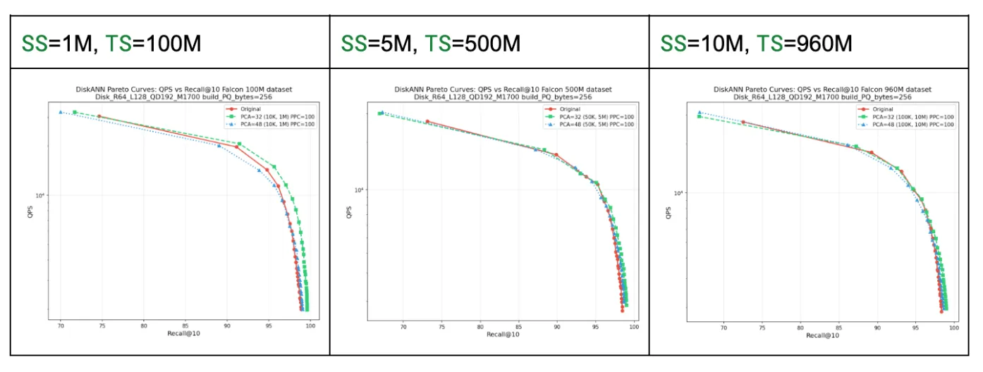
Setup: synthetic dataset generated from falcon fingerprint using the command below, compared against the real Falcon 960M and subsets on the same DiskANN build/search sweep, k=10.

$
python -m cuvs_bench.synthesize_dataset generate \
>
    --fingerprint path/to/falcon_10M_nc100000_ncomp32_fingerprint.npz \
>
    --total_rows 960000000 \
>
    --gt_mode exact \
>
    --output_dir synthetic_falcon_960M/

BigANN — synth vs real (1B, 128d)

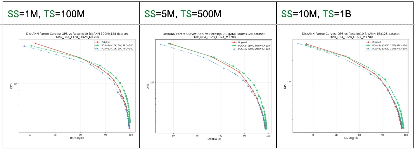
Setup: synthetic dataset generated from bigann fingerprint using the command below, compared against the real BigANN 1B and subsets on the same build/search sweep, k=10.

$
python -m cuvs_bench.synthesize_dataset generate \
>
    --fingerprint path/to/bigann_10M_nc100000_ncomp32_fingerprint.npz \
>
    --total_rows 1000000000 \
>
    --gt_mode exact \
>
    --output_dir synthetic_bigann_1B/

Wiki — synth vs real (88M, 768d)

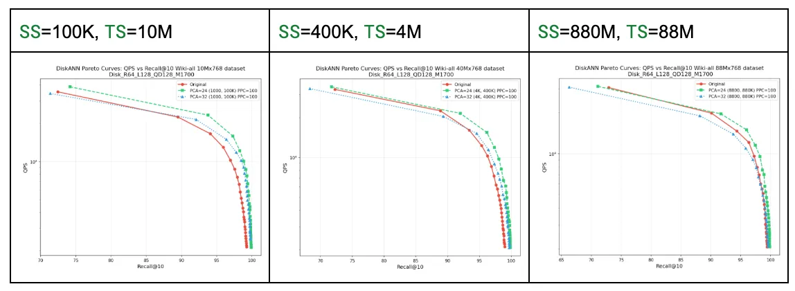
Setup: synthetic dataset generated from wiki fingerprint using the command below, compared against the real Wiki 88M and subsets on the same build/search sweep, k=10.

$
python -m cuvs_bench.synthesize_dataset generate \
>
    --fingerprint path/to/wiki_880K_nc8800_ncomp32_fingerprint.npz \
>
    --total_rows 88000000 \
>
    --gt_mode exact \
>
    --output_dir synthetic_wiki_88M/

Caveats

• The synthetic data is calibrated to reproduce how a vector index behaves on your real data (recall, throughput, build time), not the raw distance values themselves. Use it to compare index configurations, not as a substitute for distance-correctness tests.
• ncomp is the dominant parameter. Above the ceiling, recall degrades uniformly across the entire recall range.
• Queries are sampled from the synthetic distribution itself (with small noise added)

Glossary

• nc — number of KMeans clusters.
• ncomp — PCA components per cluster (the rank of the per-cluster covariance approximation).
• PPC — points per cluster in the fitting sample (= sample_size / nc). Defaults assume PPC=100, which is the empirically validated sweet spot.
• SF — scale factor (= total_rows / sample_size). How much we “stretch” the small sample to fill the target dataset.

Python API

The CLI is a thin wrapper. For programmatic use:

1
from cuvs_bench.synthesize_dataset import (
2
    Fingerprint,
3
    fit_fingerprint,
4
    save_fingerprint,
5
    load_fingerprint,
6
    generate_synthetic_dataset,
7
    generate_queries,
8
    compute_groundtruth_nprobe,
9
    compute_groundtruth_exact,
10
    verify_groundtruth,
11
)

See module docstrings for argument details.