Dynamic Mode

Optical Flow

This notebook presents how to use DALI to calculate optical flow for a given sequence of frames.

Let’s start with some handy imports

import os
from pathlib import Path

import numpy as np

import nvidia.dali.experimental.dynamic as ndd

from matplotlib import pyplot as plt

Setting metaparameters.

As an example we use Sintel trailer, included in DALI_extra repository. Feel free to verify against your own video data.

DALI_EXTRA_PATH environment variable should point to the place where data from DALI extra repository is downloaded. Please make sure that the proper release tag is checked out.

sequence_length = 10
dali_extra_dir = Path(os.environ["DALI_EXTRA_PATH"])
video_filename = str(
    dali_extra_dir
    / "db"
    / "optical_flow"
    / "sintel_trailer"
    / "sintel_trailer_short.mp4"
)

Functions used for Optical flow visualization.

The code comes from Tomrunia’s GitHub

def make_colorwheel():
    """
    Generates a color wheel for optical flow visualization as presented in:
        Baker et al. "A Database and Evaluation Methodology for Optical Flow"
        (ICCV, 2007)
        URL: http://vision.middlebury.edu/flow/flowEval-iccv07.pdf
    According to the C++ source code of Daniel Scharstein
    According to the Matlab source code of Deqing Sun
    """

    RY = 15
    YG = 6
    GC = 4
    CB = 11
    BM = 13
    MR = 6

    ncols = RY + YG + GC + CB + BM + MR
    colorwheel = np.zeros((ncols, 3))
    col = 0

    # RY
    colorwheel[0:RY, 0] = 255
    colorwheel[0:RY, 1] = np.floor(255 * np.arange(0, RY) / RY)
    col = col + RY
    # YG
    colorwheel[col : col + YG, 0] = 255 - np.floor(255 * np.arange(0, YG) / YG)
    colorwheel[col : col + YG, 1] = 255
    col = col + YG
    # GC
    colorwheel[col : col + GC, 1] = 255
    colorwheel[col : col + GC, 2] = np.floor(255 * np.arange(0, GC) / GC)
    col = col + GC
    # CB
    colorwheel[col : col + CB, 1] = 255 - np.floor(255 * np.arange(CB) / CB)
    colorwheel[col : col + CB, 2] = 255
    col = col + CB
    # BM
    colorwheel[col : col + BM, 2] = 255
    colorwheel[col : col + BM, 0] = np.floor(255 * np.arange(0, BM) / BM)
    col = col + BM
    # MR
    colorwheel[col : col + MR, 2] = 255 - np.floor(255 * np.arange(MR) / MR)
    colorwheel[col : col + MR, 0] = 255
    return colorwheel


def flow_compute_color(u, v, convert_to_bgr=False):
    """
    Applies the flow color wheel to (possibly clipped) flow components u and v.
    According to the C++ source code of Daniel Scharstein
    According to the Matlab source code of Deqing Sun
    :param u: np.ndarray, input horizontal flow
    :param v: np.ndarray, input vertical flow
    :param convert_to_bgr: bool, whether to change ordering and output BGR
                                 instead of RGB
    :return:
    """

    flow_image = np.zeros((u.shape[0], u.shape[1], 3), np.uint8)

    colorwheel = make_colorwheel()  # shape [55x3]
    ncols = colorwheel.shape[0]

    rad = np.sqrt(np.square(u) + np.square(v))
    a = np.arctan2(-v, -u) / np.pi

    fk = (a + 1) / 2 * (ncols - 1)
    k0 = np.floor(fk).astype(np.int32)
    k1 = k0 + 1
    k1[k1 == ncols] = 0
    f = fk - k0

    for i in range(colorwheel.shape[1]):
        tmp = colorwheel[:, i]
        col0 = tmp[k0] / 255.0
        col1 = tmp[k1] / 255.0
        col = (1 - f) * col0 + f * col1

        idx = rad <= 1
        col[idx] = 1 - rad[idx] * (1 - col[idx])
        col[~idx] = col[~idx] * 0.75  # out of range?

        # Note the 2-i => BGR instead of RGB
        ch_idx = 2 - i if convert_to_bgr else i
        flow_image[:, :, ch_idx] = np.floor(255 * col)

    return flow_image


def flow_to_color(flow_uv, clip_flow=None, convert_to_bgr=False):
    """
    Expects a two dimensional flow image of shape [H,W,2]
    According to the C++ source code of Daniel Scharstein
    According to the Matlab source code of Deqing Sun
    :param flow_uv: np.ndarray of shape [H,W,2]
    :param clip_flow: float, maximum clipping value for flow
    :return:
    """

    assert flow_uv.ndim == 3, "input flow must have three dimensions"
    assert flow_uv.shape[2] == 2, "input flow must have shape [H,W,2]"

    if clip_flow is not None:
        flow_uv = np.clip(flow_uv, 0, clip_flow)

    u = flow_uv[:, :, 0]
    v = flow_uv[:, :, 1]

    rad = np.sqrt(np.square(u) + np.square(v))
    rad_max = np.max(rad)

    epsilon = 1e-5
    u = u / (rad_max + epsilon)
    v = v / (rad_max + epsilon)

    return flow_compute_color(u, v, convert_to_bgr)

Using DALI

We create a video reader and call optical_flow on the video tensor to compute the optical flow.

For more information, please refer to readers.Video and optical_flow documentation.

reader = ndd.readers.Video(
    device="gpu",
    filenames=video_filename,
    sequence_length=sequence_length,
    file_list_include_preceding_frame=True,
)

video = reader()
of = ndd.optical_flow(video, output_grid=4)
of = of.cpu()
print(of.shape)

(9, 180, 320, 2)

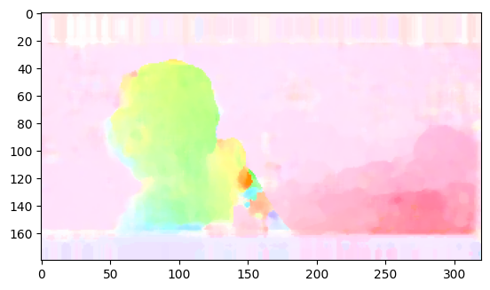
Above you can see the shape of the calculated optical flow (in FHWC format). It contains 2 channels: flow vector in x axis and flow vector in y axis. Output resolution is determined by output_grid option passed to optical_flow operator: for output_grid = 4, 4x4 grid is used for flow calculation, thus resolution in every dimension being 4 times smaller than the resolution of the input image.

Visualize Results

of_result = flow_to_color(of[sequence_length // 2])
plt.imshow(of_result)

<matplotlib.image.AxesImage at 0x7a48b470c670>