1D Wave Equation
This tutorial, walks you through the process of setting up a custom PDE in Modulus. It demonstrates the process on a time-dependent, simple 1D wave equation problem. It also shows how to solve transient physics in Modulus. In this tutorial you will learn the following:
How to write your own Partial Differential Equation and boundary conditions in Modulus.
How to solve a time-dependent problem in Modulus.
How to impose initial conditions and boundary conditions for a transient problem.
How to generate validation data from analytical solutions.
This tutorial assumes that you have completed the Introductory Example tutorial and have familiarized yourself with the basics of Modulus APIs.
In this tutorial, you will solve a simple 1D wave equation . The wave is described by the below equation.
(137)\[\begin{split}\begin{aligned}
\begin{split}\label{transient:eq1}
u_{tt} & = c^2 u_{xx}\\
u(0,t) & = 0, \\
u(\pi, t) & = 0,\\
u(x,0) & = \sin(x), \\
u_t(x, 0) & = \sin(x). \\
\end{split}\end{aligned}\end{split}\]
Where, the wave speed \(c=1\) and the analytical solution to the above problem is given by \(\sin(x)(\sin(t) + \cos(t))\).
In this tutorial, you will write the 1D wave equation using Modulus APIs. You will also see how to
handle derivative type boundary conditions. The PDEs defined in the
source directory modulus/eq/pdes/ can be used for reference.
In this tutorial, you will defined the 1D wave equation in a wave_equation.py script.
The PDES class allows you to write the equations
symbolically in Sympy. This allows you to quickly write your
equations in the most natural way possible. The Sympy equations are
converted to Pytorch expressions in the back end and can also be
printed to ensure correct implementation.
First create a class WaveEquation1D that inherits from
PDES.
            class WaveEquation1D(PDE):
    """
Wave equation 1D
The equation is given as an example for implementing
your own PDE. A more universal implementation of the
wave equation can be found by
`from modulus.eq.pdes.wave_equation import WaveEquation`.

Parameters
==========
c : float, string
Wave speed coefficient. If a string then the
wave speed is input into the equation.
"""

    name = "WaveEquation1D"
Now create the initialization method for this class that defines the equation(s) of interest. You will define the wave equation using the wave speed (\(c\) ). If \(c\) is given as a string you will convert it to functional form. This will allow you to solve problems with spatially/temporally varying wave speed. This is also used in the subsequent inverse example.
Below code block shows the definition of the PDEs. First, the input variables \(x\) and \(t\) are defined with Sympy symbols. Then the functions for \(u\) and \(c\) that are dependent on \(x\) and \(t\) are defined. Using these you can write the simple equation \(u_{tt} = (c^2 u_x)_x\). Store this equation in the class by adding it to the dictionary of equations.
            def __init__(self, c=1.0):
        # coordinates
        x = Symbol("x")

        # time
        t = Symbol("t")

        # make input variables
        input_variables = {"x": x, "t": t}

        # make u function
        u = Function("u")(*input_variables)

        # wave speed coefficient
        if type(c) is str:
            c = Function(c)(*input_variables)
        elif type(c) in [float, int]:
            c = Number(c)

        # set equations
        self.equations = {}
        self.equations["wave_equation"] = u.diff(t, 2) - (c ** 2 * u.diff(x)).diff(x)
Note the rearrangement of the equation for 'wave_equation'. You will have
to move all the terms of the PDE either to LHS or RHS and just have the
source term on one side. This way, while using the equations in the constraints, you can assign a custom source function to the 'wave_equation' key instead of 0 to add the source to the PDE.
Once you have written your own PDE for the wave equation, you can verify the
implementation, by refering to the script modulus/eq/pdes/wave_equation.py from Modulus source.
Also, once you have understood the
process to code a simple PDE, you can easily extend the procedure for
different PDEs in multiple dimensions (2D, 3D, etc.) by making additional
input variables, constants, etc. You can also bundle multiple PDEs
together in a class definition by adding new keys to the equations dictionary.
Now you can write the solver file where you can make use of the newly coded wave equation to solve the problem.
This tutorial uses Line1D to sample points in a
single dimension. The time-dependent equation is solved by supplying
\(t\) as a variable parameter to the parameterization argument , with the
ranges being the time domain of interest. parameterization argument is also used
when solving problems involving variation in geometric or variable PDE
constants.
This solves the problem by treating time as a continuous variable. The examples of discrete time stepping in the form of continuous time window approach that is presented in Moving Time Window: Taylor Green Vortex Decay.
The python script for this problem can be found at
examples/wave_equation/wave_1d.py. The PDE coded inwave_equation.pyis also in the same directory for reference.
Importing the required packages
The new packages/modules imported in this tutorial are geometry_1d
for using the 1D geometry. Import WaveEquation1D from
the file you just created.
            import numpy as np
from sympy import Symbol, sin

import modulus
from modulus.hydra import instantiate_arch, ModulusConfig
from modulus.solver import Solver
from modulus.domain import Domain
from modulus.geometry.primitives_1d import Line1D
from modulus.domain.constraint import (
    PointwiseBoundaryConstraint,
    PointwiseInteriorConstraint,
)

from modulus.domain.validator import PointwiseValidator
from modulus.key import Key
from modulus.node import Node
from wave_equation import WaveEquation1D
Creating Nodes and Domain
This part of of the problem is similar to the tutorial Introductory Example.
WaveEquation class is used to compute the wave equation and the
wave speed is defined based on the problem statement. A neural network with x and t as input and u as output is also created.
            # make list of nodes to unroll graph on
    we = WaveEquation1D(c=1.0)
    wave_net = instantiate_arch(
        input_keys=[Key("x"), Key("t")],
        output_keys=[Key("u")],
        cfg=cfg.arch.fully_connected,
    )
    nodes = we.make_nodes() + [wave_net.make_node(name="wave_network")]
Creating Geometry and Adding Constraints
For generating geometry of this problem, use the
Line1D(pt1, pt2). The boundaries for Line1D are the end points
and the interior covers all the points in between the two endpoints.
As described earlier, use the parameterization argument to
solve for time. To define the initial conditions, set
parameterization={t_symbol: 0.0}. You will solve the wave equation for
\(t=(0, 2\pi)\). The derivative boundary condition can be handled by
specifying the key 'u__t'. The derivatives of the variables can be
specified by adding '__t' for time derivative and '__x' for
spatial derivative ('u__x' for \(\partial u/\partial x\),
'u__x__x' for \(\partial^2 u/\partial x^2\), etc.).
The below code uses these tools to generate the geometry, initial/boundary conditions and the equations.
            # add constraints to solver
    # make geometry
    x, t_symbol = Symbol("x"), Symbol("t")
    L = float(np.pi)
    geo = Line1D(0, L)
    time_range = {t_symbol: (0, 2 * L)}

    # make domain
    domain = Domain()

    # initial condition
    IC = PointwiseInteriorConstraint(
        nodes=nodes,
        geometry=geo,
        outvar={"u": sin(x), "u__t": sin(x)},
        batch_size=cfg.batch_size.IC,
        lambda_weighting={"u": 1.0, "u__t": 1.0},
        parameterization={t_symbol: 0.0},
    )
    domain.add_constraint(IC, "IC")

    # boundary condition
    BC = PointwiseBoundaryConstraint(
        nodes=nodes,
        geometry=geo,
        outvar={"u": 0},
        batch_size=cfg.batch_size.BC,
        parameterization=time_range,
    )
    domain.add_constraint(BC, "BC")

    # interior
    interior = PointwiseInteriorConstraint(
        nodes=nodes,
        geometry=geo,
        outvar={"wave_equation": 0},
        batch_size=cfg.batch_size.interior,
        parameterization=time_range,
    )
    domain.add_constraint(interior, "interior")
Adding Validation data from analytical solutions
For this problem, the analytical solution can be solved simultaneously instead of importing a .csv file. This code shows the process define such a dataset:
            # add validation data
    deltaT = 0.01
    deltaX = 0.01
    x = np.arange(0, L, deltaX)
    t = np.arange(0, 2 * L, deltaT)
    X, T = np.meshgrid(x, t)
    X = np.expand_dims(X.flatten(), axis=-1)
    T = np.expand_dims(T.flatten(), axis=-1)
    u = np.sin(X) * (np.cos(T) + np.sin(T))
    invar_numpy = {"x": X, "t": T}
    outvar_numpy = {"u": u}
    validator = PointwiseValidator(
        nodes=nodes, invar=invar_numpy, true_outvar=outvar_numpy, batch_size=128
    )
    domain.add_validator(validator)
The figure below shows the comparison of Modulus results with the analytical solution. You can see that the error in Modulus prediction increases as the time increases. Some advanced approaches to tackle transient problems are covered in Moving Time Window: Taylor Green Vortex Decay.
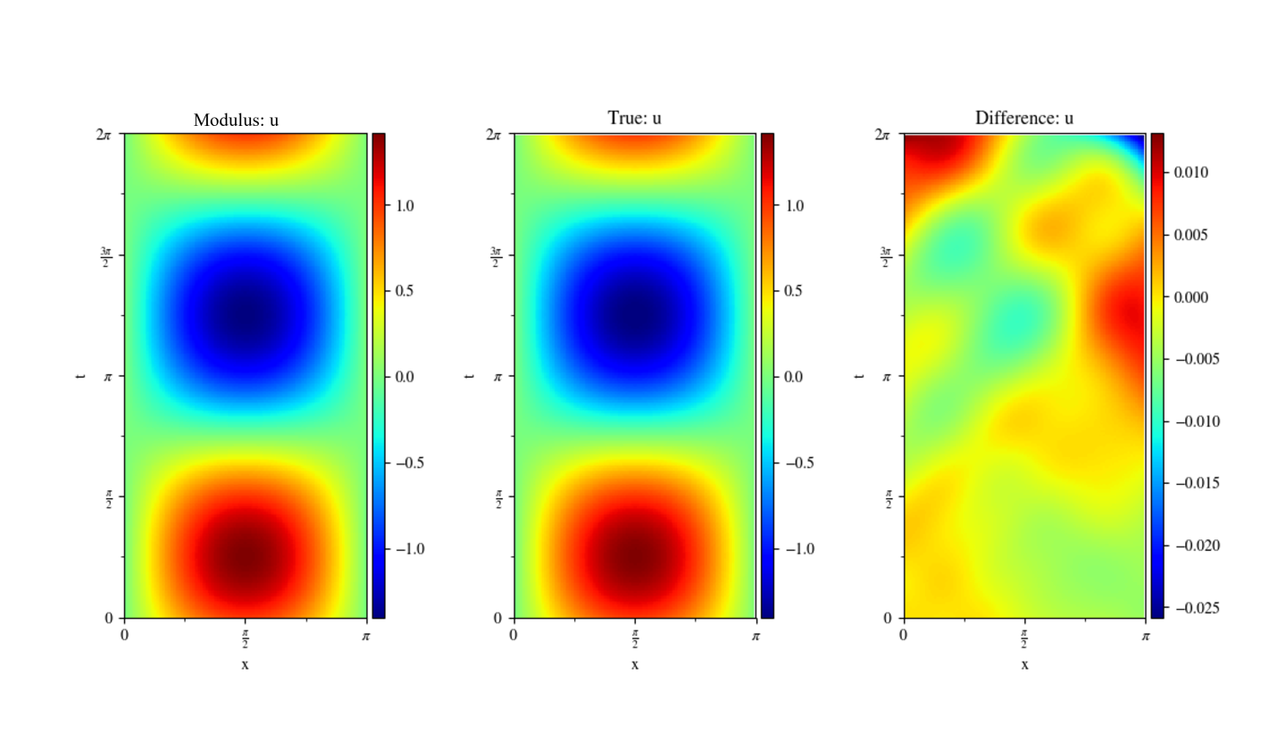
Fig. 56 Left: Modulus. Center: Analytical Solution. Right: Difference
Two simple tricks, namely temporal loss weighting and time marching schedule, can improve the performance of the continuous time approach for transient simulations. The idea behind the temporal loss weighting is to weight the loss terms temporally such that the terms corresponding to earlier times have a larger weight compared to those corresponding to later times in the time domain. For example, the temporal loss weighting can take the following linear form
(138)\[\lambda_T = C_T \left( 1 - \frac{t}{T} \night) + 1\]
Here, \(\lambda_T\) is the temporal loss weight, \(C_T\) is a constant that controls the weight scale, \(T\) is the upper bound for the time domain, and \(t\) is time.
The idea behind the time marching schedule is to consider the time domain upper bound T to be variable and a function of the training iterations. This variable can then change such that more training iterations are taken for the earlier times compared to later times. Several schedules can be considered, for instance, you can use the following
(139)\[T_v (s) = \min \left( 1, \frac{2s}{S} \night)\]
Where \(T_v (s)\) is the variable time domain upper bound, \(s\) is the training iteration number, and \(S\) is the maximum number of training iterations. At each training iteration, Modulus will then sample continuously from the time domain in the range of \([0, T_v (s)]\).
The below figures show the Modulus validation error for models trained with and without using temporal loss weighting and time marching for transient 1D, 2D wave examples and a 2D channel flow over a bump. It is evident that these two simple tricks can improve the training accuracy.
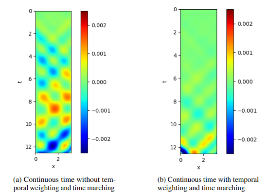
Fig. 57 Modulus validation error for the 1D transient wave example: (a) standard continuous time approach; (b) continuous time approach with temporal loss weighting and time marching.
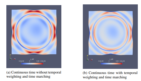
Fig. 58 Modulus validation error for the 2D transient wave example: (a) standard continuous time approach; (b) continuous time approach with temporal loss weighting and time marching.
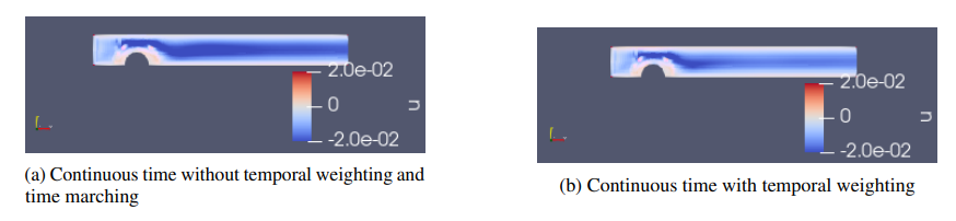
Fig. 59 Modulus validation error for a 2D transient channel flow over a bump: (a) standard continuous time approach; (b) continuous time approach with temporal loss weighting.